Note
Click here to download the full example code
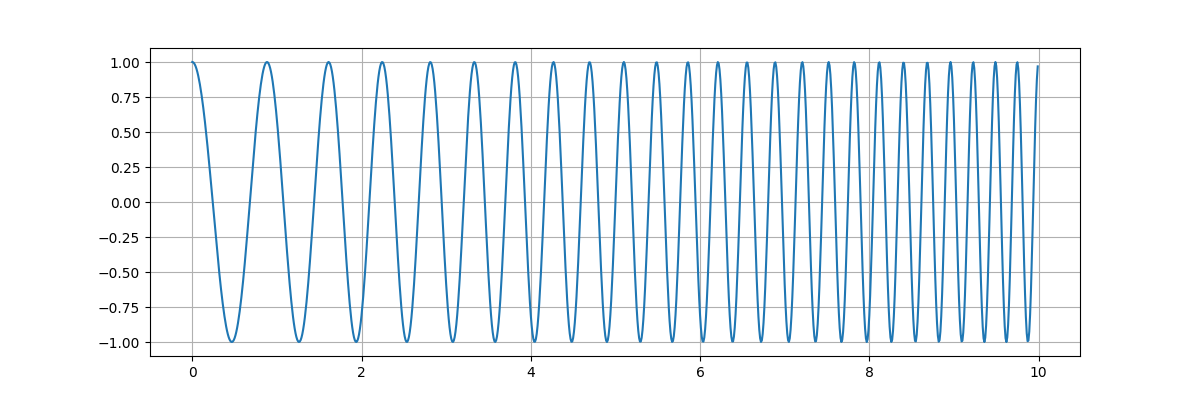
Chirp CWT with Ricker
In this example, we analyze a chirp signal with a Ricker (a.k.a. Mexican Hat wavelet)
# Configure JAX to work with 64-bit floating point precision.
from jax.config import config
config.update("jax_enable_x64", True)
Let’s import necessary libraries
import numpy as np
import jax.numpy as jnp
# CR.Sparse libraries
import cr.sparse as crs
import cr.sparse.wt as wt
# Utilty functions to construct sinusoids
import cr.sparse.dsp.signals as signals
# Plotting
import matplotlib.pyplot as plt
Test signal generation
Sampling frequency in Hz
fs = 100
# Signal duration in seconds
T = 10
# Initial instantaneous frequency for the chirp
f0 = 1
# Final instantaneous frequency for the chirp
f1 = 4
# Construct the chirp signal
t, x = signals.chirp(fs, T, f0, f1, initial_phase=0)
# Plot the chirp signal
fig, ax = plt.subplots(figsize=(12, 4))
ax.plot(t, x)
ax.grid('on')
Power spectrum
# Compute the power spectrum
f, sxx = crs.power_spectrum(x, dt=1/fs)
# Plot the power spectrum
fig, ax = plt.subplots(1, figsize=(12,4))
ax.plot(f, sxx)
ax.grid('on')
ax.set_xlabel('Frequency (Hz)')
ax.set_ylabel('Power')

Out:
Text(99.59722222222221, 0.5, 'Power')
As expected, the power spectrum is able to identify the frequencies in the zone 1Hz to 4Hz in the chirp. However, the spectrum is unable to localize the changes in frequency over time.
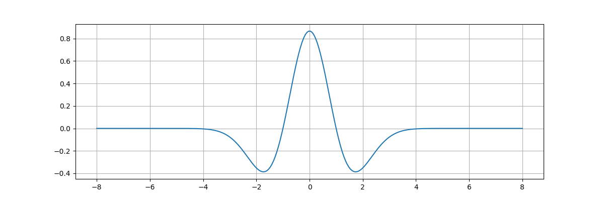
Ricker/Mexican Hat Wavelet
wavelet = wt.build_wavelet('mexh')
# generate the wavelet function for the range of time [-8, 8]
psi, t_psi = wavelet.wavefun()
# plot the wavelet
fig, ax = plt.subplots(figsize=(12, 4))
ax.plot(t_psi, psi)
ax.grid('on')
Wavelet Analysis
select a set of scales for wavelet analysis voices per octave
nu = 8
scales = wt.scales_from_voices_per_octave(nu, jnp.arange(32))
# Compute the wavelet analysis
output = wt.cwt(x, scales, wavelet)
# Identify the frequencies for the analysis
frequencies = wt.scale2frequency(wavelet, scales) * fs
# Plot the analysis
cmap = plt.cm.seismic
fig, ax = plt.subplots(1, figsize=(10,10))

title = 'Wavelet Transform (Power Spectrum) of signal'
ylabel = 'Frequency (Hz)'
xlabel = 'Time'

power = (abs(output)) ** 2
levels = [0.0625, 0.125, 0.25, 0.5, 1, 2, 4, 8]
contourlevels = np.log2(levels)

im = ax.contourf(t, jnp.log2(frequencies), jnp.log2(power), contourlevels, extend='both',cmap=cmap)

ax.set_title(title, fontsize=20)
ax.set_ylabel(ylabel, fontsize=18)
ax.set_xlabel(xlabel, fontsize=18)

yticks = 2**np.arange(np.ceil(np.log2(frequencies.min())), np.ceil(np.log2(frequencies.max())))
ax.set_yticks(np.log2(yticks))
ax.set_yticklabels(yticks)
ylim = ax.get_ylim()

Total running time of the script: ( 0 minutes 4.512 seconds)