Alternating direction algorithms for l1 problems in compressive sensing
We provide a port of YALL1 basic package. This is built on top of JAX and can be used to solve the following \(\ell_1\) minimization problems.
The basis pursuit problem
The L1/L2 minimization or basis pursuit denoising problem
The L1 minimization problem with L2 constraints
We also support corresponding non-negative counter-parts.
The nonnegative basis pursuit problem
The nonnegative L1/L2 minimization or basis pursuit denoising problem
The nonnegative L1 minimization problem with L2 constraints
In the above, \(W\) is a sparsifying basis s.t. \(Wx = \alpha\) is a sparse representation of \(x\) in \(W\) given by \(\alpha = W^T x\). For simple examples, we can assume \(W=I\) is the identity basis.
The \(\| \cdot \|_{w,1}\) is the weighted L1 (semi-) norm defined as
for a given non-negative weight vector \(w\). In the simplest case, we assume \(w=1\) reducing it to the famous \(\ell_1\) norm.
Import relevant libraries
[1]:
from jax.config import config
config.update("jax_enable_x64", True)
import jax
import jax.numpy as jnp
import numpy as np
from jax import random
from jax import jit, grad, vmap
norm = jnp.linalg.norm
[2]:
import cr.nimble as crn
import cr.sparse as crs
import cr.sparse.dict as crdict
import cr.sparse.data as crdata
import cr.sparse.lop as lop
from cr.sparse.cvx.adm import yall1
WARNING:absl:No GPU/TPU found, falling back to CPU. (Set TF_CPP_MIN_LOG_LEVEL=0 and rerun for more info.)
[3]:
import matplotlib as mpl
import matplotlib.pyplot as plt
%matplotlib inline
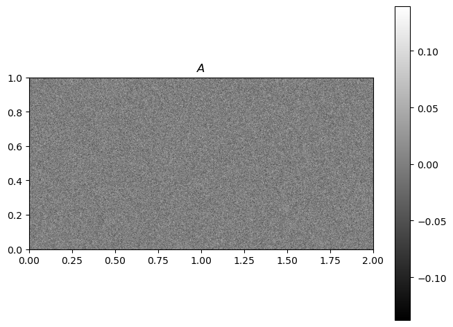
Setup a problem with a random sensing matrix with orthonormal rows
[4]:
N = 1000
M = 300
K = 50
[5]:
key = random.PRNGKey(0)
key1, key2, key3, key4 = random.split(key, 4)
[6]:
A = crdict.random_orthonormal_rows(key1, M, N)
[7]:
crn.has_orthogonal_rows(A)
[7]:
DeviceArray(True, dtype=bool)
[8]:
fig=plt.figure(figsize=(8,6), dpi= 100, facecolor='w', edgecolor='k')
plt.imshow(A, extent=[0, 2, 0, 1])
plt.gray()
plt.colorbar()
plt.title(r'$A$');
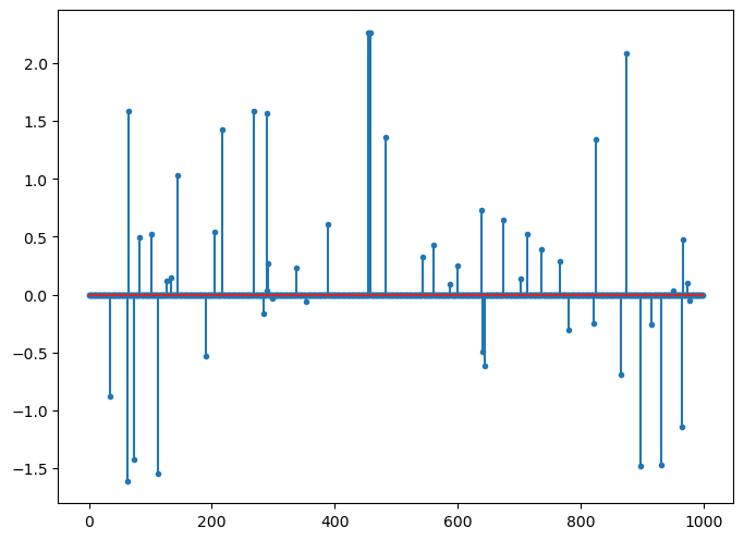
[9]:
x, omega = crdata.sparse_normal_representations(key2, N, K, 1)
x = jnp.squeeze(x)
[10]:
fig=plt.figure(figsize=(8,6), dpi= 100, facecolor='w', edgecolor='k')
plt.stem(x, markerfmt='.');
[11]:
# Convert A into a linear operator
A = lop.matrix(A)
Standard sparse recovery problems for compressive sensing
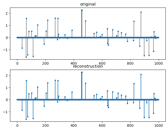
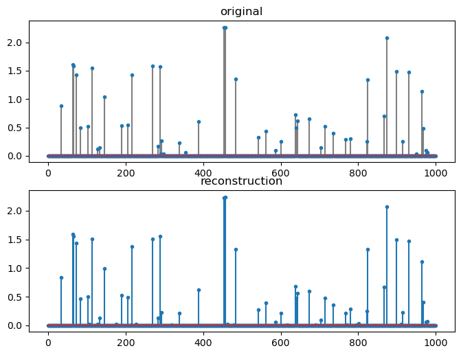
Basis pursuit
The simple form of basis pursuit problem is:
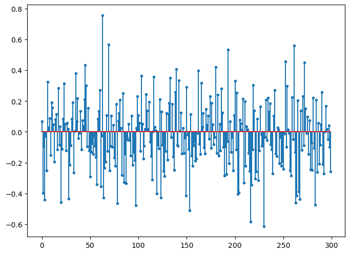
[12]:
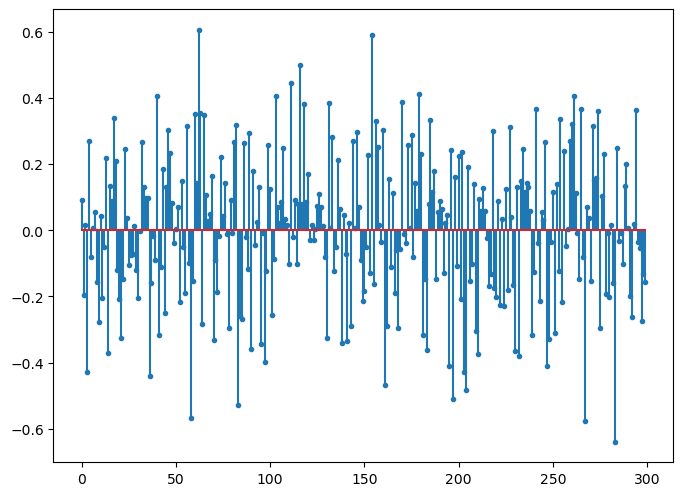
# Compute the measurements
b0 = A.times(x)
[13]:
fig=plt.figure(figsize=(8,6), dpi= 100, facecolor='w', edgecolor='k')
plt.stem(b0, markerfmt='.');
[14]:
sol = yall1.solve(A, b0)
[15]:
print(sol)
iterations 30
n_times 61
n_trans 32
r_norm 3.658499e-02
[16]:
crn.signal_noise_ratio(x, sol.x)
[16]:
DeviceArray(38.35395527, dtype=float64)
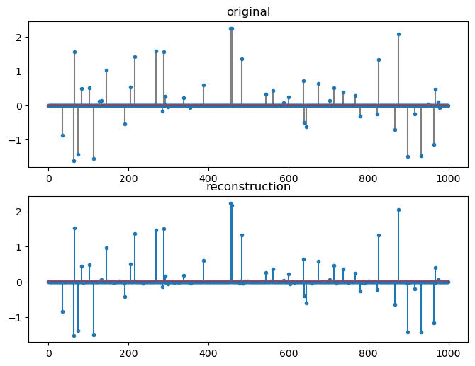
[17]:
fig=plt.figure(figsize=(8,6), dpi= 100, facecolor='w', edgecolor='k')
plt.subplot(211)
plt.title('original')
plt.stem(x, markerfmt='.', linefmt='gray');
plt.subplot(212)
plt.stem(sol.x, markerfmt='.');
plt.title('reconstruction');
[18]:
%timeit yall1.solve(A, b0).x.block_until_ready()
5.66 ms ± 702 µs per loop (mean ± std. dev. of 7 runs, 100 loops each)
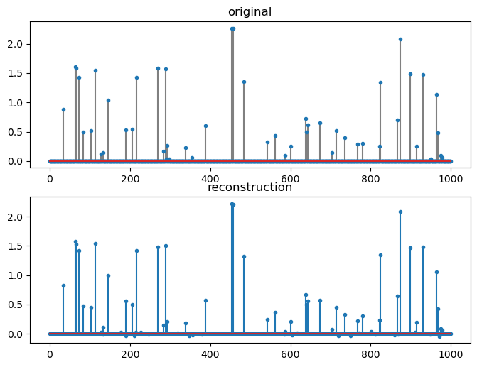
Basis pursuit denoising
The simple form of L1-L2 unconstrained minimization or basis pursuit denoising is:
[19]:
sigma = 0.01
noise = sigma * random.normal(key3, (M,))
[20]:
b = b0 + noise
[21]:
crn.signal_noise_ratio(b0, b)
[21]:
DeviceArray(27.34386008, dtype=float64)
[22]:
sol = yall1.solve(A, b, rho=0.01)
print(sol)
iterations 28
n_times 57
n_trans 30
r_norm 1.781138e-01
[23]:
crn.signal_noise_ratio(x, sol.x)
[23]:
DeviceArray(23.82452563, dtype=float64)
[24]:
fig=plt.figure(figsize=(8,6), dpi= 100, facecolor='w', edgecolor='k')
plt.subplot(211)
plt.title('original')
plt.stem(x, markerfmt='.', linefmt='gray');
plt.subplot(212)
plt.stem(sol.x, markerfmt='.');
plt.title('reconstruction');
[25]:
%timeit yall1.solve(A, b, rho=0.01).x.block_until_ready()
6.37 ms ± 604 µs per loop (mean ± std. dev. of 7 runs, 100 loops each)
Basis pursuit with inequality constraints
The simple form of L1 minimization with L2 constraints or basis pursuit with inequality constraints is:
[26]:
delta = float(norm(noise))
delta
[26]:
0.16467458902598492
[27]:
sol = yall1.solve(A, b, delta=delta)
print(sol)
iterations 26
n_times 53
n_trans 28
r_norm 1.868910e-01
[28]:
crn.signal_noise_ratio(x, sol.x)
[28]:
DeviceArray(23.58768603, dtype=float64)
[29]:
fig=plt.figure(figsize=(8,6), dpi= 100, facecolor='w', edgecolor='k')
plt.subplot(211)
plt.title('original')
plt.stem(x, markerfmt='.', linefmt='gray');
plt.subplot(212)
plt.stem(sol.x, markerfmt='.');
plt.title('reconstruction');

[30]:
%timeit yall1.solve(A, b, delta=delta).x.block_until_ready()
6.96 ms ± 712 µs per loop (mean ± std. dev. of 7 runs, 100 loops each)
Non-negative counterparts
In this case, the signal \(x\) with the sparse representation \(\alpha = W x\) has only non-negative entries. i.e. if an entry in \(x\) is non-zero, it is positive. This is typical for images.
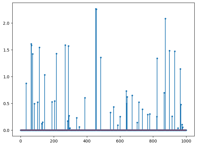
Let us construct a sparse representation with non-negative entries.
[31]:
xp = jnp.abs(x)
[32]:
fig=plt.figure(figsize=(8,6), dpi= 100, facecolor='w', edgecolor='k')
plt.stem(xp, markerfmt='.');
Non-negative basis pursuit
The simple form of basis pursuit for non-negative \(x\) is:
[33]:
b0p = A.times(xp)
[34]:
fig=plt.figure(figsize=(8,6), dpi= 100, facecolor='w', edgecolor='k')
plt.stem(b0p, markerfmt='.');
[35]:
sol = yall1.solve(A, b0p, nonneg=True)
print(sol)
iterations 36
n_times 73
n_trans 38
r_norm 2.969753e-02
[36]:
crn.signal_noise_ratio(xp, sol.x)
[36]:
DeviceArray(39.20630974, dtype=float64)
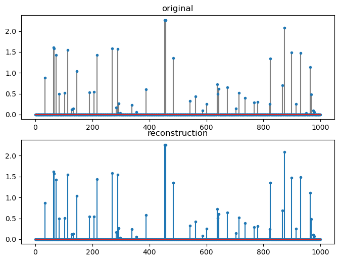
[37]:
fig=plt.figure(figsize=(8,6), dpi= 100, facecolor='w', edgecolor='k')
plt.subplot(211)
plt.title('original')
plt.stem(xp, markerfmt='.', linefmt='gray');
plt.subplot(212)
plt.stem(sol.x, markerfmt='.');
plt.title('reconstruction');
[38]:
%timeit yall1.solve(A, b0p, nonneg=True).x.block_until_ready()
8.3 ms ± 511 µs per loop (mean ± std. dev. of 7 runs, 100 loops each)
Non-negative basis pursuit denoising
The simple form of L1-L2 unconstrained minimization with non-negative \(x\) is:
[39]:
bp = b0p + noise
[40]:
crs.signal_noise_ratio(b0p, bp)
[40]:
DeviceArray(27.43652935, dtype=float64)
[41]:
sol = yall1.solve(A, bp, nonneg=True, rho=0.01)
print(sol)
iterations 28
n_times 57
n_trans 30
r_norm 1.898381e-01
[42]:
crs.signal_noise_ratio(xp, sol.x)
[42]:
DeviceArray(27.55570803, dtype=float64)
[43]:
fig=plt.figure(figsize=(8,6), dpi= 100, facecolor='w', edgecolor='k')
plt.subplot(211)
plt.title('original')
plt.stem(xp, markerfmt='.', linefmt='gray');
plt.subplot(212)
plt.stem(sol.x, markerfmt='.');
plt.title('reconstruction');
[44]:
%timeit yall1.solve(A, bp, nonneg=True, rho=0.01).x.block_until_ready()
6.48 ms ± 793 µs per loop (mean ± std. dev. of 7 runs, 100 loops each)
Non-negative basis pursuit with inequality constraints
[45]:
sol = yall1.solve(A, bp, delta=delta)
print(sol)
iterations 24
n_times 49
n_trans 26
r_norm 1.915944e-01
[46]:
crs.signal_noise_ratio(xp, sol.x)
[46]:
DeviceArray(25.37898646, dtype=float64)
[47]:
fig=plt.figure(figsize=(8,6), dpi= 100, facecolor='w', edgecolor='k')
plt.subplot(211)
plt.title('original')
plt.stem(xp, markerfmt='.', linefmt='gray');
plt.subplot(212)
plt.stem(sol.x, markerfmt='.');
plt.title('reconstruction');
[48]:
%timeit yall1.solve(A, bp, delta=delta).x.block_until_ready()
6.37 ms ± 334 µs per loop (mean ± std. dev. of 7 runs, 100 loops each)
