Dirac Cosine Dictionaries
![]()
In this tutorial we will:
Construct a Cosine basis
Construct a Dirac-Cosine dictionary.
Construct a signal which is a mixture of few impulses and a few sinusoids.
Construct its representation in the Cosine basis.
Recover its representation in Dirac-Cosine dictionary using following sparse recovery algorithms
Orthogonal Matching Pursuit
Measure the recovery error for different sparse recovery algorithms.
[1]:
# Make sure that cr-sparse package is available on colab
!python -m pip install --quiet git+https://github.com/carnotresearch/cr-sparse.git
We use JAX for numerical computations. Importing JAX dependencies:
[2]:
import jax
import jax.numpy as jnp
Importing relevant modules from the CR-Sparse library:
[3]:
import cr.sparse as crs
import cr.sparse.dict as crdict
import cr.sparse.pursuit as pursuit
We will use matplotlib for all visualizations in this notebook.
[4]:
import matplotlib as mpl
import matplotlib.pyplot as plt
[5]:
%matplotlib inline
We will be working with signals in the space \(\mathbb{R}^M\). The dimension of signal space:
[6]:
M = 256
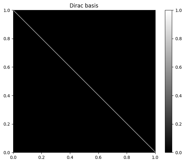
The standard basis or identity basis or Dirac basis for the signal space \(I \in \mathbb{R}^{M \times M}\) can be easily constructed using JAX:
[7]:
I = jnp.eye(M)
fig=plt.figure(figsize=(8,6), dpi= 100, facecolor='w', edgecolor='k')
plt.imshow(I, extent=[0, 1, 0, 1])
plt.gray()
plt.colorbar()
plt.title(r'Dirac basis');
WARNING:absl:No GPU/TPU found, falling back to CPU. (Set TF_CPP_MIN_LOG_LEVEL=0 and rerun for more info.)
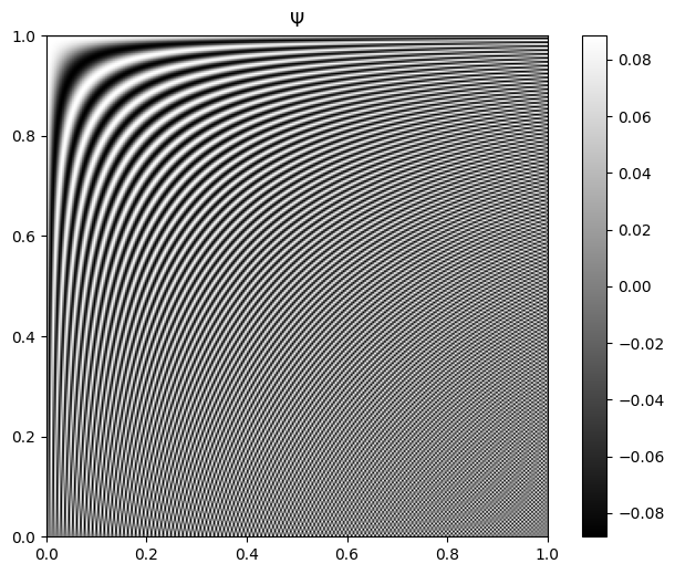
Cosine basis construction
[8]:
Psi = crdict.cosine_basis(M)
Psi.shape
[8]:
(256, 256)
Visualizing the Cosine basis
[9]:
fig=plt.figure(figsize=(8,6), dpi= 100, facecolor='w', edgecolor='k')
plt.imshow(Psi, extent=[0, 1, 0, 1])
plt.gray()
plt.colorbar()
plt.title(r'$\Psi$');
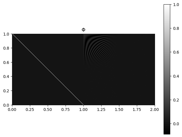
Dirac-Cosine dictionary construction
A Dirac-Cosine dictionary is a concatenation of the two orthonormal bases (the Dirac basis and the Cosine basis). A simple way to do the same using Jax is:
[10]:
jnp.hstack([I, Psi]);
CR-Sparse provides a ready-made method for constructing a Dirac-Cosine dictionary for \(\mathbb{R}^M\):
[11]:
Phi = crdict.dirac_cosine_basis(M)
As expected, the number of atoms in this dictionary is twice of \(M\):
[12]:
Phi.shape
[12]:
(256, 512)
[13]:
N = Phi.shape[1]
N
[13]:
512
We can say that the dictionary \(\Phi\) maps representations in \(\mathbb{R}^N\) to signals in \(\mathbb{R}^M\). \(\mathbb{R}^N\) is called the representation space and \(\mathbb{R}^M\) is called the signal space.
Visualizing the Dirac-Cosine dictionary:
[14]:
fig=plt.figure(figsize=(8,6), dpi= 100, facecolor='w', edgecolor='k')
plt.imshow(Phi, extent=[0, 2, 0, 1])
plt.gray()
plt.colorbar()
plt.title(r'$\Phi$');
A mixture signal of impulses and sinusoids
We can combine some of the atoms from the Dirac basis and some of the atoms from the Cosine basis, alternatively, some atoms from Dirac-Cosine dictionary to form a signal which is a mixture of impulses and sinusoids. The atoms from Dirac basis contribute the impulses and the atoms from the Dirac basis contribute the sinusoids.
[15]:
x = crs.build_signal_from_indices_and_values(N, [20, 30, 100, M+3, M+57], [1, -0.4, 0.6, 1.2, -0.8])
y = Phi @ x
Visualizing the mixture signal
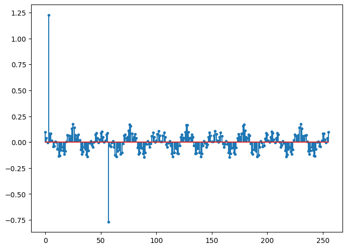
[16]:
fig=plt.figure(figsize=(8,6), dpi= 100, facecolor='w', edgecolor='k')
plt.stem(y, markerfmt='.', use_line_collection=True);
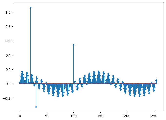
Notice the three impulses. The periodic component is coming from the two sinusoids.
\(x\) in the equation \(y = \Phi x\) above is the sparse representation of \(y\) in the dictionary \(\Phi\). It is called a sparse representation as it consists of very few non-zero values corresponding to the atoms which contribute in the construction of \(y\). CR-Sparse provides some convenient functions to extrat the non-zero indices and non-zero values of a sparse representation.
The support \(I\) of the representation \(x\):
[17]:
crs.nonzero_indices(x)
[17]:
DeviceArray([ 20, 30, 100, 259, 313], dtype=int32)
The non-zero entries in \(x\) over \(I\) a.k.a. \(x_I\):
[18]:
crs.nonzero_values(x)
[18]:
DeviceArray([ 1. , -0.4, 0.6, 1.2, -0.8], dtype=float32)
We remind that we can write \(y = \Phi x\) as \(y = \Phi_I x_I\) too as atoms with zero contribution in \(y\) can be removed from the computation.
Mixture signal representation in Cosine basis
The representation of a signal \(y\) in an orthogonal basis \(\Psi\) is constructed by computing \(\Psi^T y\). Let’s see how does our \(y\) fare in the Cosine basis:
[19]:
y_Cosine = Psi.T @ y
[20]:
fig=plt.figure(figsize=(8,6), dpi= 100, facecolor='w', edgecolor='k')
plt.stem(y_Cosine, markerfmt='.', use_line_collection=True);
We can see that there are two impulses in the Cosine basis representation of \(y\) which correspond to the sinusoids present in \(y\). However, it also consists of a mix of sinusoids which are the representation of the impulses in \(y\) in the Cosine basis. Thus, the representation of \(y\) in the Cosine basis \(\Psi\) is not sparse. In fact, \(y\) doesn’t have a sparse representation in any orthonormal basis for \(\mathbb{R}^M\).
Building a sparse representation in the Dirac Cosine basis
Constructing the representation of \(y\) in a dictionary is a non-trivial problem as it is an overcomplete set of atoms. There are infinite possible representations of \(y\) in \(\Phi\). However, under suitable conditions, the sparse representation of \(y\) in \(\Phi\) is unique. Also, under suitable conditions, there exist algorithms which can recover the sparse representation of \(y\) in \(\Phi\).
One class of algorithms is called greedy pursuit algorithms. A representative in this class is Orthogonal Matching Pursuit (OMP). In order to run this algorithm, it is imperative that we are aware of the number of non-zero entries in the sparse representation (a.k.a. the sparsity of the representation of \(y\) in \(\Phi\)). Fortunatley, in this example, we know this trivially:
[21]:
K = crs.nonzero_indices(x).size
K
[21]:
5
CR-Sparse provides a ready-made implementation of OMP. Let’s import the module which provides this functionality.
[22]:
import cr.sparse.pursuit.omp
Running the OMP sparse recovery algorithm:
[23]:
solution = pursuit.omp.solve(Phi, y, K)
In order to save space, the algorithm returns the nonzero values and their indices in the sparse representation:
The values at non-zero entries in the representation \(x_I\):
[24]:
solution.x_I
[24]:
DeviceArray([ 1.1999999 ,  1.        , -0.7999999 ,  0.59999996,
             -0.39999998], dtype=float32)
The indices of non-zero entries \(I\):
[25]:
solution.I
[25]:
DeviceArray([259, 20, 313, 100, 30], dtype=int32)
Note that the indices as identified by OMP may not be in the same order as earlier. The order of indices doesn’t matter.
CR-Sparse provides a convenient function to combine the non-zero indices and values to form the overall sparse representation in \(\mathbb{R}^N\).
[26]:
z = crs.build_signal_from_indices_and_values(N, solution.I, solution.x_I)
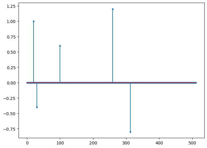
Visualizing the representation:
[27]:
fig=plt.figure(figsize=(8,6), dpi= 100, facecolor='w', edgecolor='k')
plt.stem(z, markerfmt='.', use_line_collection=True);
Sparse representation error
In general, OMP may be fed a signal \(y = \Phi x + e\) where \(e\) is the sparse representation error. When OMP estimates \(x\) is actually computes an approximation \(\hat{x}\). It also estimates a residual \(r = y - \Phi \hat{x}\).
The energy of the residual is given by:
[28]:
solution.r_norm_sqr
[28]:
DeviceArray(3.802608e-14, dtype=float32)
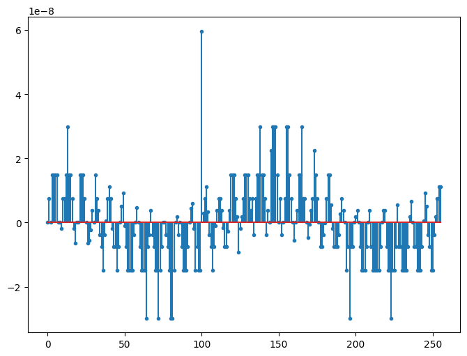
In this case, the energy of residual is very small as there was no representation error in the original computation \(y = \Phi x\). This residual energy corresponds to floating point computation errors.
Visualizing the residual:
[29]:
fig=plt.figure(figsize=(8,6), dpi= 100, facecolor='w', edgecolor='k')
plt.stem(solution.r, markerfmt='.', use_line_collection=True);
[ ]:
