Blocks Signal in Haar Basis

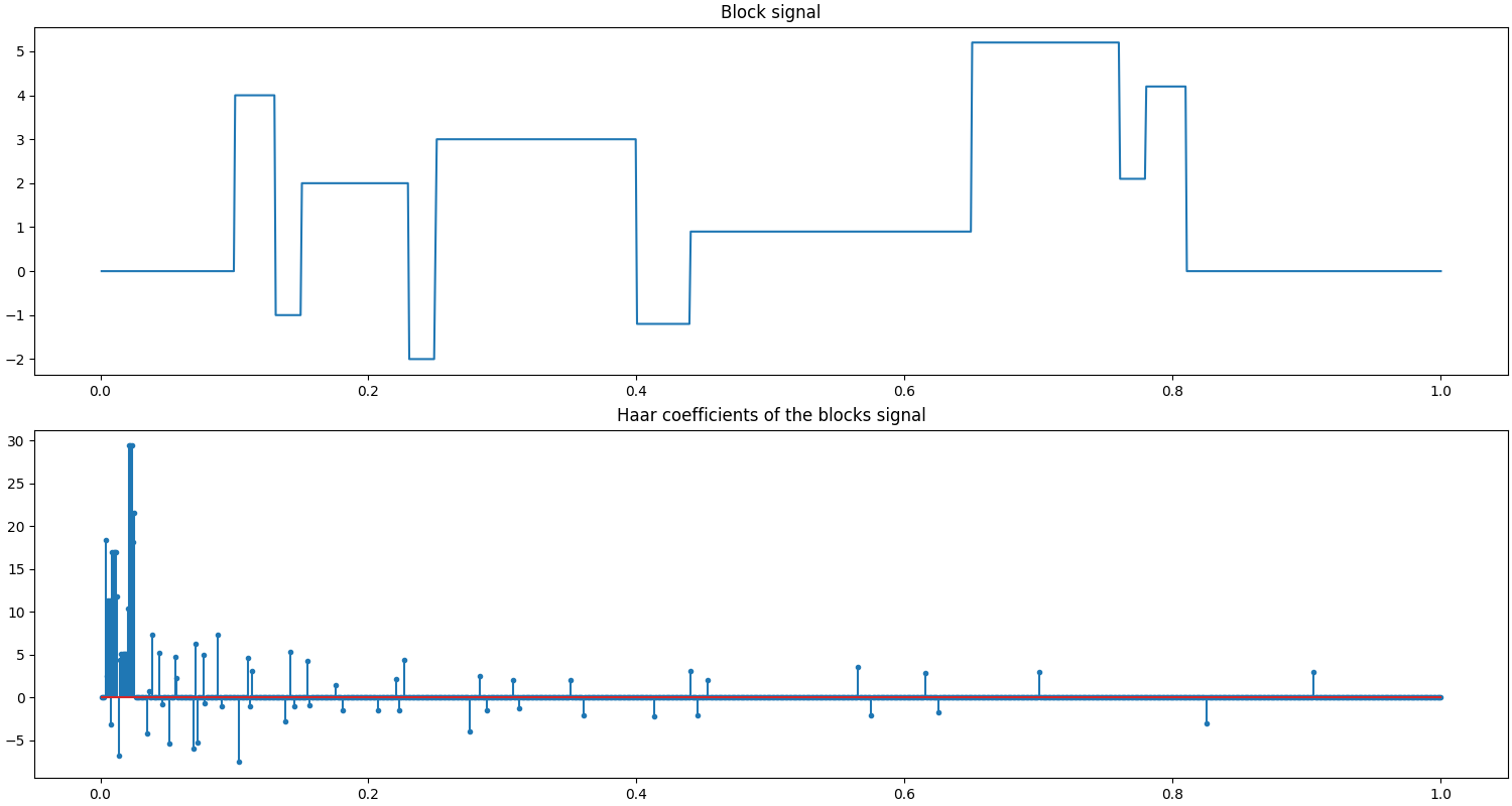
A Blocks signal as proposed by Donoho et al. in Wavelab [BD95] is a concatenation of blocks with different heights. It has a sparse representation in a Haar basis.

In this test problem with the structure \(\bb = \bA \bx\), the signal \(\bb\) is the blocks signal (of length 1024), \(\bA\) is a Haar basis with 5 levels of decomposition and \(\bx\) is the sparse representation of the signal in this basis. This basis is real, complete and orthonormal. Hence, a simple solution for getting \(\bx\) from \(\bb\) is the formula:

(1)\[\bx = \bA^T \bb.\]

This test problem is useful in identifying basic mistakes in a sparse recovery algorithm. This problem should be very easy to solve by any sparse recovery algorithm. However, there is a caveat. If a sparse recovery algorithm depends on the expected sparsity of the signal (typically a parameter K in greedy algorithms), the reconstruction would fail if K is specified below the actual number of significant components of \(\bx\).

See also:

• Test Problems

• Linear Operators

# Configure JAX to work with 64-bit floating point precision.
from jax.config import config
config.update("jax_enable_x64", True)

import jax.numpy as jnp
import cr.nimble as crn
import cr.sparse as crs
import cr.sparse.plots as crplot

Setup

We shall construct our test signal and dictionary using our test problems module.

from cr.sparse import problems
prob = problems.generate('blocks:haar')
fig, ax = problems.plot(prob)

Let us access the relevant parts of our test problem

# The sparsifying basis linear operator
A = prob.A
# The Blocks signal
b0 = prob.b
# The sparse representation of the Blocks signal in the dictionary
x0 = prob.x

Check how many coefficients in the sparse representation are sufficient to capture 99.9% of the energy of the signal

print(crn.num_largest_coeffs_for_energy_percent(x0, 99.9))

64

This number gives us an idea about the required sparsity to be configured for greedy pursuit algorithms.

Sparse Recovery using Subspace Pursuit

We shall use subspace pursuit to reconstruct the signal.

import cr.sparse.pursuit.sp as sp
# We will try to estimate a 100-sparse representation
sol = sp.solve(A, b0, 100)

This utility function helps us quickly analyze the quality of reconstruction

problems.analyze_solution(prob, sol)

m: 1024, n: 1024
b_norm: original: 78.899 reconstruction: 78.899 SNR: 289.74 dB
x_norm: original: 78.899 reconstruction: 78.899 SNR: 135.52 dB
Sparsity: original: 64, reconstructed: 64, overlap: 64, ratio: 1.000
Iterations: 1

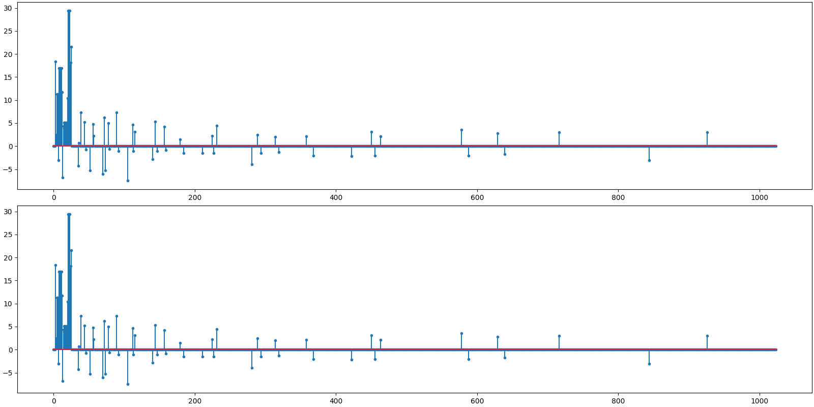
The estimated sparse representation

x = sol.x

Let us reconstruct the signal from this sparse representation

b = prob.reconstruct(x)

Let us visualize the original and reconstructed representation

ax = crplot.h_plots(2)
ax[0].stem(x0, markerfmt='.')
ax[1].stem(x, markerfmt='.')

<StemContainer object of 3 artists>

Let us visualize the original and reconstructed signal

ax = crplot.h_plots(2)
ax[0].plot(b0)
ax[1].plot(b)

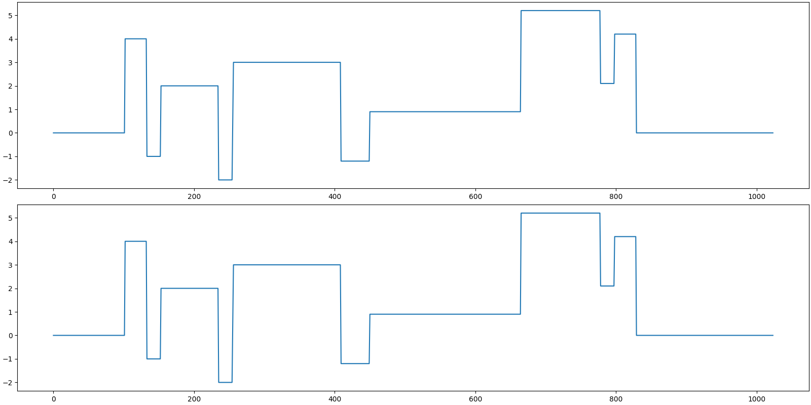
[<matplotlib.lines.Line2D object at 0x7f27d0587e20>]

Sparse Recovery using Compressive Sampling Matching Pursuit

We shall now use compressive sampling matching pursuit to reconstruct the signal.

import cr.sparse.pursuit.cosamp as cosamp
# We will try to estimate a 100-sparse representation
sol = cosamp.solve(A, b0, 100)
problems.analyze_solution(prob, sol)

m: 1024, n: 1024
b_norm: original: 78.899 reconstruction: 78.899 SNR: 289.03 dB
x_norm: original: 78.899 reconstruction: 78.899 SNR: 135.52 dB
Sparsity: original: 64, reconstructed: 64, overlap: 64, ratio: 1.000
Iterations: 2

The estimated sparse representation

x = sol.x

Let us reconstruct the signal from this sparse representation

b = prob.reconstruct(x)

Let us visualize the original and reconstructed representation

ax = crplot.h_plots(2)
ax[0].stem(x0, markerfmt='.')
ax[1].stem(x, markerfmt='.')

<StemContainer object of 3 artists>

Let us visualize the original and reconstructed signal

ax = crplot.h_plots(2)
ax[0].plot(b0)
ax[1].plot(b)

[<matplotlib.lines.Line2D object at 0x7f27d06e4430>]

Sparse Recovery using SPGL1

import cr.sparse.cvx.spgl1 as crspgl1
options = crspgl1.SPGL1Options()
tracker = crs.ProgressTracker(x0=x0)
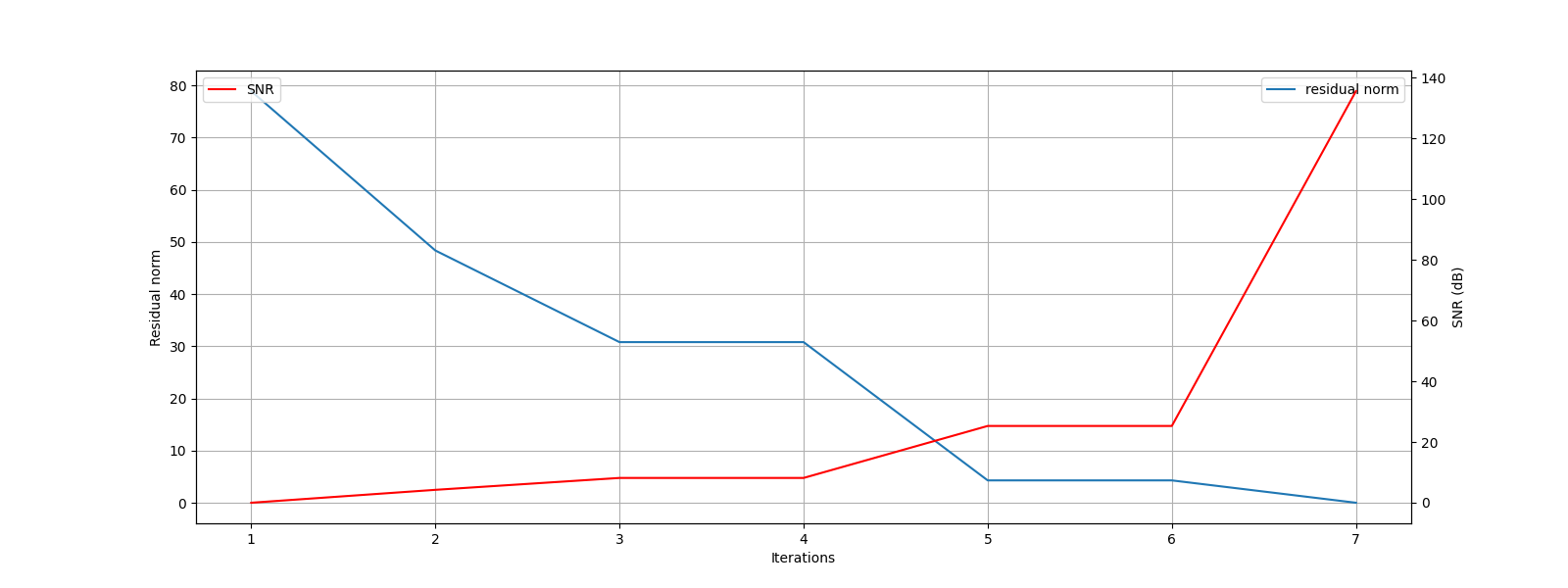
sol = crspgl1.solve_bp_jit(A, b0, options=options, tracker=tracker)

[1] x_norm: 0.00e+00, r_norm: 7.89e+01, SNR: 0.00 dB
[2] x_norm: 3.05e+01, r_norm: 4.84e+01, SNR: 4.25 dB
[3] x_norm: 5.74e+01, r_norm: 3.08e+01, SNR: 8.17 dB
[4] x_norm: 5.74e+01, r_norm: 3.08e+01, SNR: 8.17 dB
[5] x_norm: 7.61e+01, r_norm: 4.28e+00, SNR: 25.30 dB
[6] x_norm: 7.61e+01, r_norm: 4.28e+00, SNR: 25.30 dB
[7] x_norm: 7.89e+01, r_norm: 2.48e-07, SNR: 135.63 dB
Algorithm converged in 7 iterations.

Let’s analyze the solution quality

problems.analyze_solution(prob, sol)

m: 1024, n: 1024
b_norm: original: 78.899 reconstruction: 78.899 SNR: 170.06 dB
x_norm: original: 78.899 reconstruction: 78.899 SNR: 135.63 dB
Sparsity: original: 64, reconstructed: 64, overlap: 64, ratio: 1.000
Iterations: 7 n_times: 10, n_trans: 8

Let’s plot the progress of SPGL1 over different iterations

ax = crplot.one_plot(height=6)
tracker.plot_progress(ax)

The estimated sparse representation

x = sol.x

Let us reconstruct the signal from this sparse representation

b = prob.reconstruct(x)

Let us visualize the original and reconstructed representation

ax = crplot.h_plots(2)
ax[0].stem(x0, markerfmt='.')
ax[1].stem(x, markerfmt='.')

<StemContainer object of 3 artists>

Let us visualize the original and reconstructed signal

ax = crplot.h_plots(2)
ax[0].plot(b0)
ax[1].plot(b)

[<matplotlib.lines.Line2D object at 0x7f27b7456ac0>]

Comments

We note that SP converges in a single iteration, CoSaMP takes two iterations, while SPGL1 takes 9 iterations to converge.