Complex Sinusoids+Complex-Spikes in Dirac-Fourier Basis

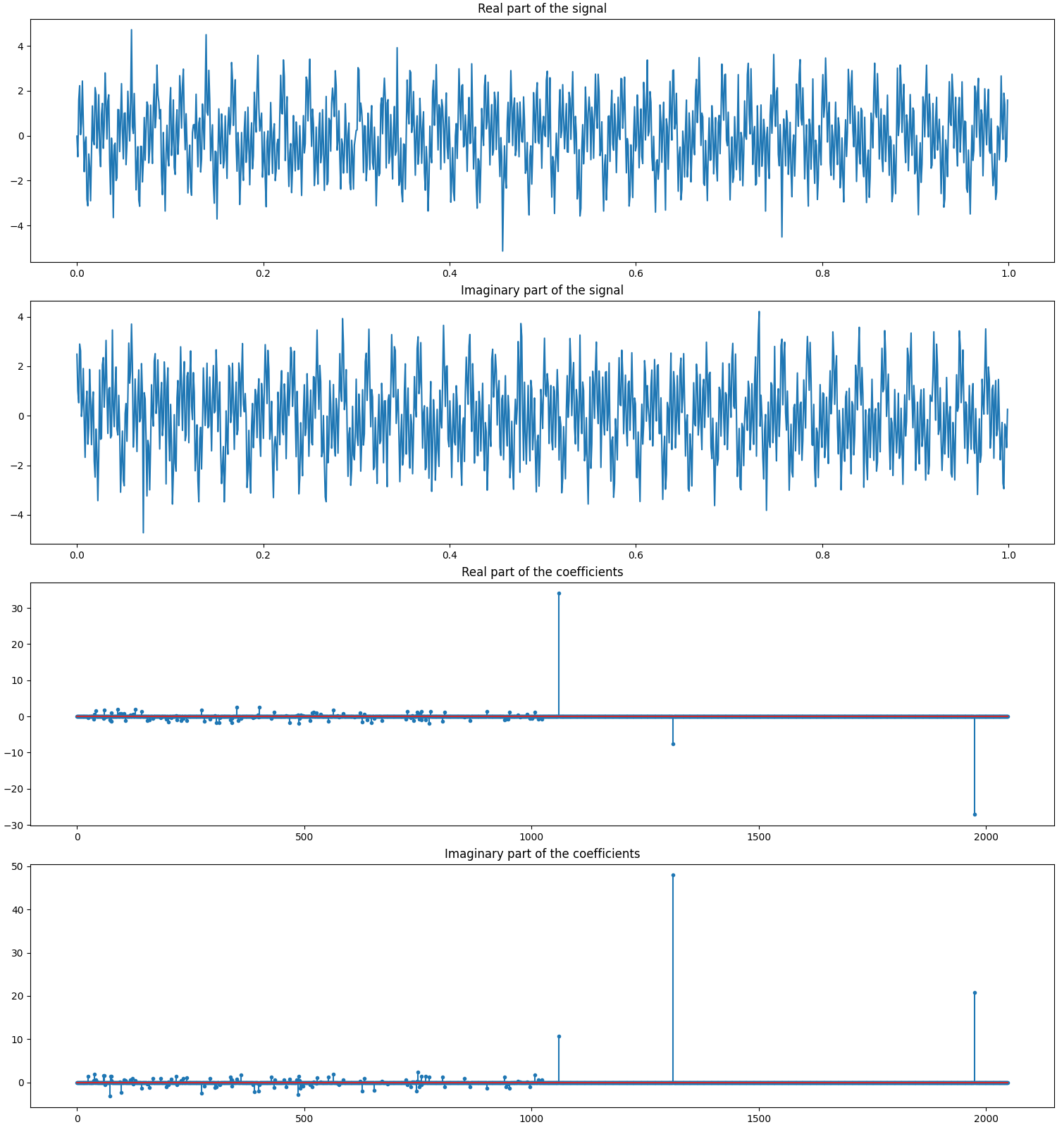
The Complex Sinusoids+Spikes signal in this example consists of a mixture of 3 different complex sinusoids with different amplitudes/phases and 120 different complex spikes (with normally distributed amplitudes for both real and imaginary parts and randomly chosen locations).

The sinusoid part of the signal has a sparse representation in the Fourier basis. The Spikes part of the signal has a sparse representation in the Dirac(Identity/Standard) basis. Thus, the mixture Sinusoid+Spikes signal has a sparse representation (of 123 nonzero coefficients) in the Dirac-Fourier two ortho basis.

Note that the spikes are normally distributed. Some of the spikes have extremely low amplitudes. They may be missed by a recovery algorithm depending on convergence thresholds.

See also:

• Test Problems

• Linear Operators

# Configure JAX to work with 64-bit floating point precision.
from jax.config import config
config.update("jax_enable_x64", True)

import jax.numpy as jnp
import cr.nimble as crn
import cr.sparse.plots as crplot

Setup

We shall construct our test signal and dictionary using our test problems module.

from cr.sparse import problems
prob = problems.generate('complex:sinusoid-spikes:dirac-fourier', c=3, k=120)
fig, ax = problems.plot(prob)

Let us access the relevant parts of our test problem

# The sparsifying basis linear operator
A = prob.A
# The Complex Sinusoids+Spikes signal
b0 = prob.b
# The sparse representation of the signal in the dictionary
x0 = prob.x

Check how many coefficients in the sparse representation are sufficient to capture 99.9% of the energy of the signal

print(crn.num_largest_coeffs_for_energy_percent(x0, 99.9))

102

This number gives us an idea about the required sparsity to be configured for greedy pursuit algorithms.

Sparse Recovery using Subspace Pursuit

We shall use subspace pursuit to reconstruct the signal.

import cr.sparse.pursuit.sp as sp

# We will first try to estimate a 100-sparse representation
sol = sp.solve(A, b0, 100)

This utility function helps us quickly analyze the quality of reconstruction

problems.analyze_solution(prob, sol)

m: 1024, n: 2048
b_norm: original: 71.089 reconstruction: 71.047 SNR: 29.32 dB
x_norm: original: 71.188 reconstruction: 71.241 SNR: 29.29 dB
Sparsity: original: 102, reconstructed: 93, overlap: 93, ratio: 0.912
Iterations: 20

It takes 20 iterations to converge and 76 of the largest 78 entries have been correctly identified.

We will now try to estimate a 150-sparse representation

sol = sp.solve(A, b0, 150)
problems.analyze_solution(prob, sol)

m: 1024, n: 2048
b_norm: original: 71.089 reconstruction: 71.089 SNR: 293.43 dB
x_norm: original: 71.188 reconstruction: 71.188 SNR: 293.70 dB
Sparsity: original: 102, reconstructed: 102, overlap: 102, ratio: 1.000
Iterations: 3

We have correctly detected all the 78 most significant entries Let us check if we correctly decoded all the nonzero entries in the sparse representation x

problems.analyze_solution(prob, sol, perc=100)

m: 1024, n: 2048
b_norm: original: 71.089 reconstruction: 71.089 SNR: 293.43 dB
x_norm: original: 71.188 reconstruction: 71.188 SNR: 293.70 dB
Sparsity: original: 123, reconstructed: 123, overlap: 123, ratio: 1.000
Iterations: 3

The estimated sparse representation

x = sol.x

Let us reconstruct the signal from this sparse representation

b = prob.reconstruct(x)

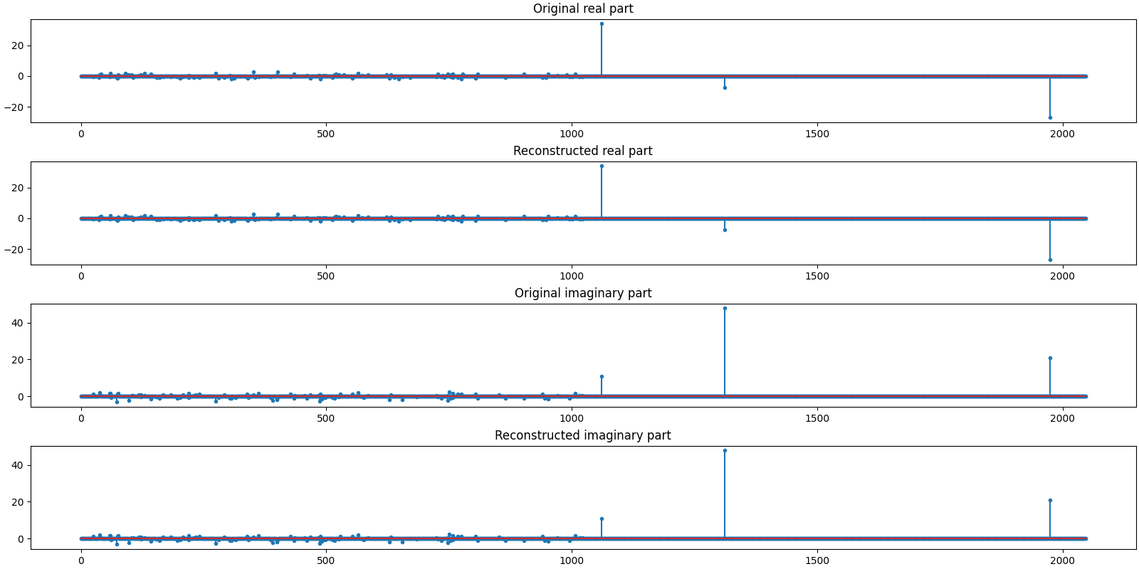
Let us visualize the original and reconstructed representation

def plot_representations(x0, x):
    ax = crplot.h_plots(4, height=2)
    ax[0].stem(jnp.real(x0), markerfmt='.')
    ax[0].set_title('Original real part')
    ax[1].stem(jnp.real(x), markerfmt='.')
    ax[1].set_title('Reconstructed real part')
    ax[2].stem(jnp.imag(x0), markerfmt='.')
    ax[2].set_title('Original imaginary part')
    ax[3].stem(jnp.imag(x), markerfmt='.')
    ax[3].set_title('Reconstructed imaginary part')
plot_representations(x0, x)

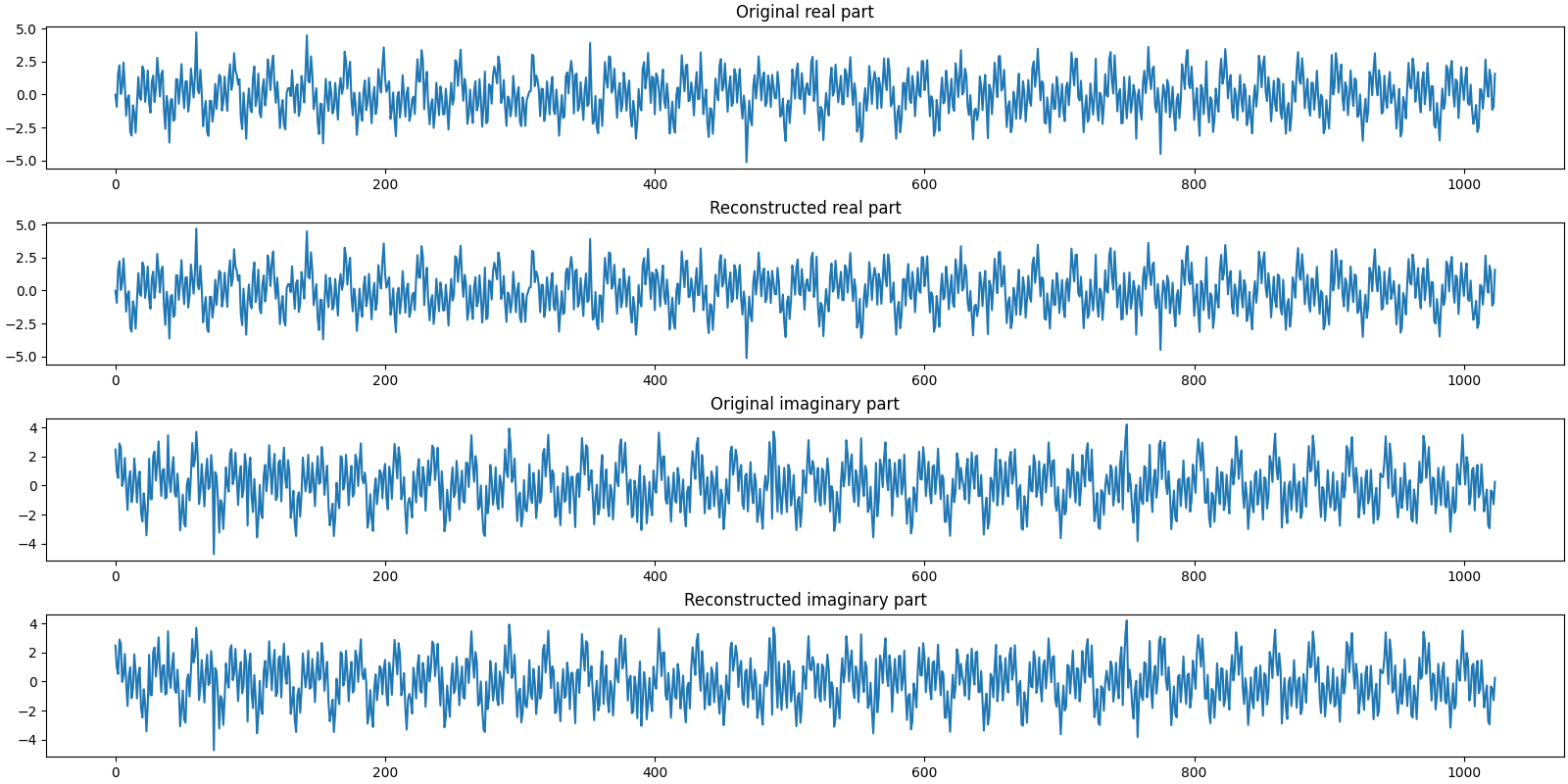
Let us visualize the original and reconstructed signal

def plot_signals(b0, b):
    ax = crplot.h_plots(4, height=2)
    ax[0].plot(jnp.real(b0))
    ax[0].set_title('Original real part')
    ax[1].plot(jnp.real(b))
    ax[1].set_title('Reconstructed real part')
    ax[2].plot(jnp.imag(b0))
    ax[2].set_title('Original imaginary part')
    ax[3].plot(jnp.imag(b))
    ax[3].set_title('Reconstructed imaginary part')
plot_signals(b0, b)

Sparse Recovery using Compressive Sampling Matching Pursuit

We shall now use compressive sampling matching pursuit to reconstruct the signal.

import cr.sparse.pursuit.cosamp as cosamp
# We will try to estimate a 150-sparse representation
sol = cosamp.solve(A, b0, 150)
problems.analyze_solution(prob, sol, perc=100)

m: 1024, n: 2048
b_norm: original: 71.089 reconstruction: 71.089 SNR: 292.93 dB
x_norm: original: 71.188 reconstruction: 71.188 SNR: 292.70 dB
Sparsity: original: 123, reconstructed: 123, overlap: 123, ratio: 1.000
Iterations: 4

The estimated sparse representation

x = sol.x

Let us reconstruct the signal from this sparse representation

b = prob.reconstruct(x)

Let us visualize the original and reconstructed representation

plot_representations(x0, x)

Let us visualize the original and reconstructed signal

plot_signals(b0, b)

Sparse Recovery using SPGL1

import cr.sparse.cvx.spgl1 as crspgl1
options = crspgl1.SPGL1Options()
sol = crspgl1.solve_bp_jit(A, b0, options=options)
problems.analyze_solution(prob, sol, perc=100)

m: 1024, n: 2048
b_norm: original: 71.089 reconstruction: 71.089 SNR: 118.43 dB
x_norm: original: 71.188 reconstruction: 71.188 SNR: 113.81 dB
Sparsity: original: 123, reconstructed: 123, overlap: 123, ratio: 1.000
Iterations: 41 n_times: 44, n_trans: 42

The estimated sparse representation

x = sol.x

Let us reconstruct the signal from this sparse representation

b = prob.reconstruct(x)

Let us visualize the original and reconstructed representation

plot_representations(x0, x)

Let us visualize the original and reconstructed signal

plot_signals(b0, b)

Comments

• With K=100, SP recovery is slightly inaccurate. It also takes more iterations to converge.

• Both SP and CoSaMP correctly recover the signal in 3 iterations if the sparsity is specified properly (150 > 123).

• SPGL1 converges in 41 iterations but correctly discovers the support without requiring any input about expected sparsity.