Note
Go to the end to download the full example code
Cosine+Spikes, Dirac-Cosine Basis, Gaussian Measurements
In this example we have
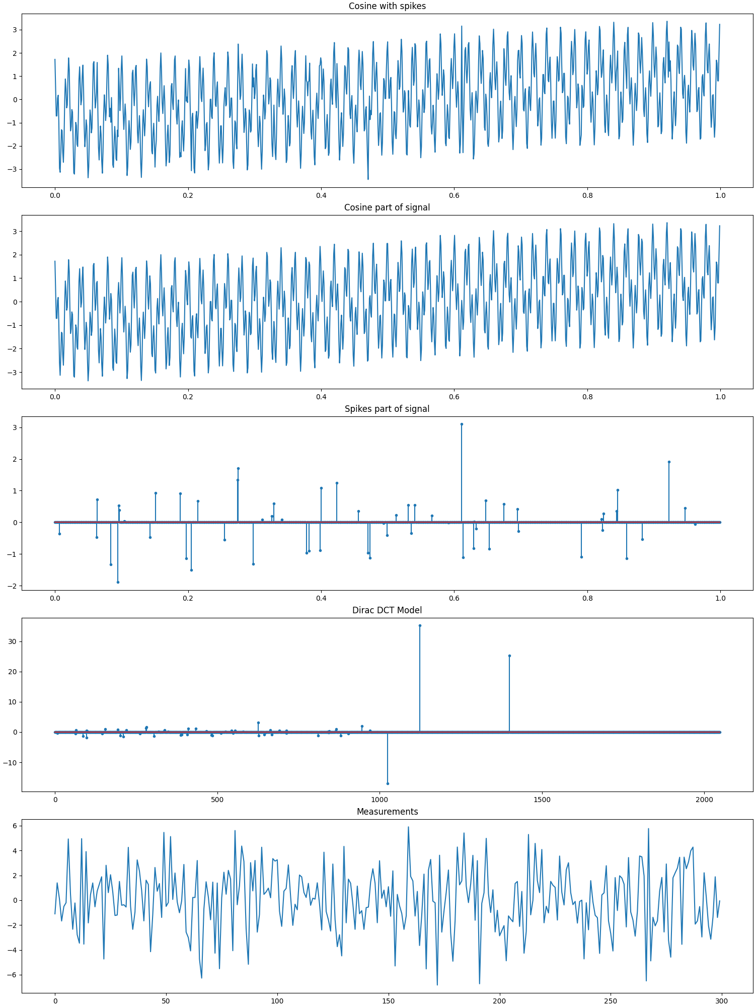
A signal \(\by\) consisting of a mixture of 3 cosine waves and 60 random spikes of total length 1024.
A Dirac-Cosine two ortho basis \(\Psi\) of shape 1024x2048.
The sparse representation \(\bx\) of the signal \(\by\) in the basis \(\Psi\) consisting of exactly 63 nonzero entries (corresponding to the spikes and the amplitudes of the cosine waves).
A Gaussian sensing matrix \(\Phi\) of shape 300x1024 making 300 random measurements in a vector \(\bb\).
We are given \(\bb\) and \(\bA = \Phi \Psi\) and have to reconstruct \(\bx\) using it.
Then we can use \(\Psi\) to compute \(\by = \Psi \bx\).
See also:
# Configure JAX to work with 64-bit floating point precision.
from jax.config import config
config.update("jax_enable_x64", True)

import jax.numpy as jnp
import cr.nimble as crn
import cr.sparse.plots as crplot
Setup
We shall construct our test signal and dictionary using our test problems module.
Let us access the relevant parts of our test problem
# The combined linear operator (sensing matrix + dictionary)
A = prob.A
# The sparse representation of the signal in the dictionary
x0 = prob.x
# The Cosine+Spikes signal
y0 = prob.y
# The measurements
b0 = prob.b
Check how many coefficients in the sparse representation are sufficient to capture 99.9% of the energy of the signal
print(crn.num_largest_coeffs_for_energy_percent(x0, 99.9))
37
This number gives us an idea about the required sparsity to be configured for greedy pursuit algorithms. Although the exact sparsity of this representation is 63 but several of the spikes are too small and could be ignored for a reasonably good approximation.
Sparse Recovery using Subspace Pursuit
We shall use subspace pursuit to reconstruct the signal.
import cr.sparse.pursuit.sp as sp

# We will first try to estimate a 50-sparse representation
sol = sp.solve(A, b0, 50)
This utility function helps us quickly analyze the quality of reconstruction
problems.analyze_solution(prob, sol)
m: 300, n: 2048
b_norm: original: 43.984 reconstruction: 43.982 SNR: 40.62 dB
x_norm: original: 47.155 reconstruction: 47.147 SNR: 39.24 dB
y_norm: original: 46.969 reconstruction: 46.986 SNR: 39.26 dB
Sparsity: original: 37, reconstructed: 36, overlap: 36, ratio: 0.973
Iterations: 20
We will now try to estimate a 75-sparse representation
sol = sp.solve(A, b0, 75)
problems.analyze_solution(prob, sol)
m: 300, n: 2048
b_norm: original: 43.984 reconstruction: 43.984 SNR: 82.42 dB
x_norm: original: 47.155 reconstruction: 47.155 SNR: 79.39 dB
y_norm: original: 46.969 reconstruction: 46.969 SNR: 79.58 dB
Sparsity: original: 37, reconstructed: 37, overlap: 37, ratio: 1.000
Iterations: 10
Let us check if we correctly decoded all the nonzero entries in the sparse representation x
problems.analyze_solution(prob, sol, perc=100)
m: 300, n: 2048
b_norm: original: 43.984 reconstruction: 43.984 SNR: 82.42 dB
x_norm: original: 47.155 reconstruction: 47.155 SNR: 79.39 dB
y_norm: original: 46.969 reconstruction: 46.969 SNR: 79.58 dB
Sparsity: original: 63, reconstructed: 75, overlap: 62, ratio: 0.827
Iterations: 10
The estimated sparse representation
x = sol.x
Let us reconstruct the signal from this sparse representation
y = prob.reconstruct(x)
The estimated measurements
b = A.times(x)
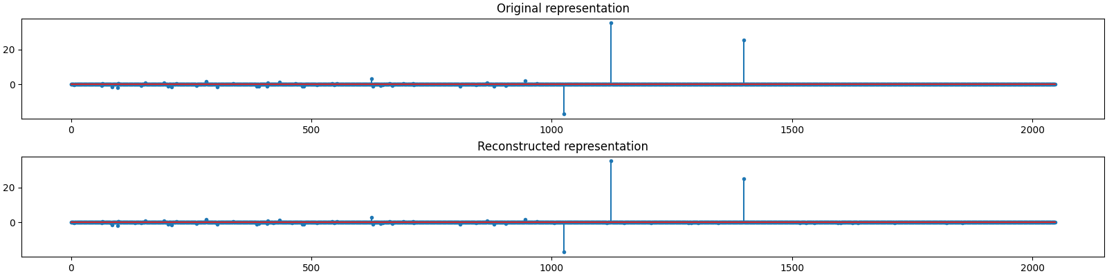
Let us visualize the original and reconstructed representation
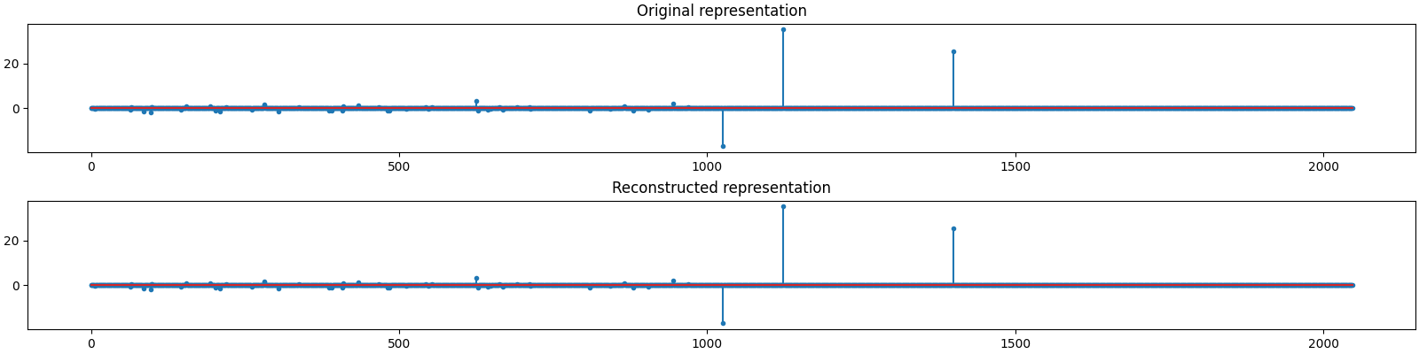
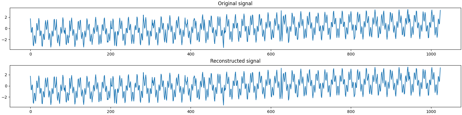
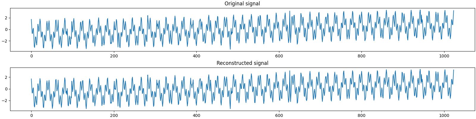
Let us visualize the original and reconstructed signal

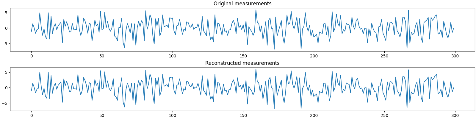
Let us visualize the original and reconstructed measurements
Sparse Recovery using Compressive Sampling Matching Pursuit
We shall now use compressive sampling matching pursuit to reconstruct the signal.
import cr.sparse.pursuit.cosamp as cosamp
# We will try to estimate a 75-sparse representation
sol = cosamp.solve(A, b0, 75)
problems.analyze_solution(prob, sol, perc=100)
m: 300, n: 2048
b_norm: original: 43.984 reconstruction: 43.984 SNR: 80.55 dB
x_norm: original: 47.155 reconstruction: 47.155 SNR: 76.81 dB
y_norm: original: 46.969 reconstruction: 46.969 SNR: 77.09 dB
Sparsity: original: 63, reconstructed: 75, overlap: 62, ratio: 0.827
Iterations: 57
The estimated sparse representation
x = sol.x
Let us reconstruct the signal from this sparse representation
y = prob.reconstruct(x)
The estimated measurements
b = A.times(x)
Let us visualize the original and reconstructed representation
plot_representations(x0, x)

Let us visualize the original and reconstructed signal
plot_signals(y0, y)
Let us visualize the original and reconstructed measurements
plot_measurments(b0, b)

Sparse Recovery using SPGL1
import cr.sparse.cvx.spgl1 as crspgl1
options = crspgl1.SPGL1Options(max_iters=1000)
sol = crspgl1.solve_bp_jit(A, b0, options=options)
problems.analyze_solution(prob, sol)
m: 300, n: 2048
b_norm: original: 43.984 reconstruction: 43.984 SNR: 112.91 dB
x_norm: original: 47.155 reconstruction: 46.907 SNR: 35.83 dB
y_norm: original: 46.969 reconstruction: 46.781 SNR: 36.82 dB
Sparsity: original: 37, reconstructed: 34, overlap: 34, ratio: 0.919
Iterations: 861 n_times: 1522, n_trans: 862
The estimated sparse representation
x = sol.x
Let us reconstruct the signal from this sparse representation
y = prob.reconstruct(x)
The estimated measurements
b = A.times(x)
Let us visualize the original and reconstructed representation
plot_representations(x0, x)
Let us visualize the original and reconstructed signal
plot_signals(y0, y)
Let us visualize the original and reconstructed measurements
plot_measurments(b0, b)


Comments
With K=50, SP recovery is slightly inaccurate. It also takes more (20) iterations to converge.
With K=75, SP is pretty good. It only missed one of the 63 nonzero entries. Also, SP converges in just 10 iterations.
With K=75, CoSaMP is also good but slightly poor. It also missed just one nonzero entry. But it seems like it missed a more significant entry compared to SP. Also, CoSaMP took 57 iterations to converge.
SPGL1 converges in 788 iterations to converge. Its model space and signal space SNR are not good. However, its measurement space SNR is pretty high.
Total running time of the script: (0 minutes 15.886 seconds)
Download Python source code: 0005.pyDownload Jupyter notebook: 0005.ipynbGallery generated by Sphinx-Gallery