Note
Go to the end to download the full example code
Deconvolution
This example demonstrates following features:
cr.sparse.lop.convolveA 1D convolution linear operatorcr.sparse.geo.rickerRicker waveletcr.sparse.sls.lsqrLSQR algorithm for solving a least square problem
Doconvolution is an inverse operation to the convolution operation. Convolving a signal with some filter may introduce some artifacts. A successful deconvolution can remove those artificats.
When a signal is observed through an instrument, an instrument usually has its own impulse response which may be spread over time. Thus, the output of the instrument will not be the original signal but a filtered version of it.
Let \(h\) denote the filter response of an instrument and \(x\) denote the signal being observed. Then the actual observation is
where \(\star\) is the convolution operation.
It is possible to model the convolution operation as a matrix multiplication.
where \(H\) is a sparse and structured matrix with non-zero entries from the impulse response \(h\).
Under this model, recovering the original signal \(x\) from the measurements \(y\) reduces to the problem of solving a sparse linear system
We can use the LSQR algorithm (available in cr.sparse.sls.lsqr) to solve this
system efficiently. LSQR algorithm doesn’t need to know the matrix \(H\)
explicitly. All it needs are two functions to compute the matrix multiplication
\(H v\) and the adjoint multiplication \(H^T u\).
We model \(H\) using the cr.sparse.lop.convolve operator.
Let’s import necessary libraries
import jax.numpy as jnp
# For plotting diagrams
import matplotlib.pyplot as plt
## CR-Sparse modules
import cr.nimble as cnb
# Linear operators
from cr.sparse import lop
# Geophysics stuff [Ricker wavelet]
from cr.sparse import geo
# DSP utilities
from cr.nimble import dsp
# Solvers for sparse linear systems
from cr.sparse import sls
# Configure JAX for 64-bit computing
from jax.config import config
config.update("jax_enable_x64", True)
Problem Setup
The Ricker wavelet response of the instrument
The time duration of the instrument response
T_h = 0.8
# Wavelet peak frequency
f0 = 30
# Time values at which the wavelet will be evaluated
t_h = dsp.time_values(fs, T_h, initial_time=-T_h/2, endpoint=True)
# Values of the Ricker wavelet
h = geo.ricker(t_h, f0)
# Plot the wavelet
fig, ax = plt.subplots(1, 1, figsize=(10, 3), dpi= 100, facecolor='w', edgecolor='k')
ax.plot(t_h, h)
# Zoom in to the central part of interest
ax.set_xlim(-0.2, 0.2)
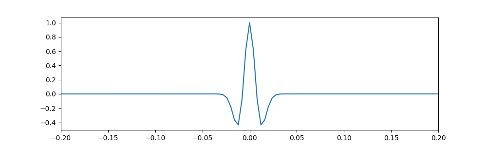
(-0.2, 0.2)
The impulse signal to be observed
T = 4
t = dsp.time_values(fs, T, endpoint=True)
# The length of the signal
n = len(t)
mid = n // 2
# A unit vector with one at mid position and zero everywhere else
x = cnb.vec_unit(n, mid)
fig, ax = plt.subplots(1,1, figsize=(10, 3), dpi= 100, facecolor='w', edgecolor='k')
ax.plot(t, x)
# Let's focus on the middle part of the signal
ax.set_xlim(1.9, 2.1)
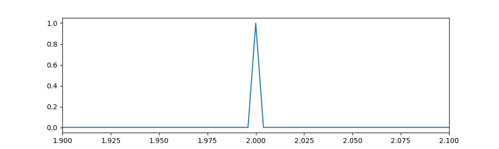
(1.9, 2.1)
The linear operator representing the instrument
Identify the peak of the impulse response
idx = jnp.argmax(jnp.abs(h))
# Construct a convolution operator based on the wavelet response
# centered at the peak of the wavelet
H = lop.convolve(n, h, offset=idx)
# JIT compile the convolution operator for efficiency
H = lop.jit(H)
The measurement process
Compute the measured signal via convolution
y = H.times(x)
# plot the original signal vs. the observed signal
fig, ax = plt.subplots(1, 1, figsize=(10, 3))
ax.plot(t, x, 'k', lw=2, label=r'$x$')
ax.plot(t, y, 'r', lw=2, label=r'$y=A x$')
ax.set_title('Signal vs Measurements', fontsize=14, fontweight='bold')
ax.legend()
# Focus on the middle part
ax.set_xlim(1.9, 2.1)
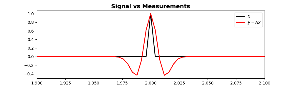
(1.9, 2.1)
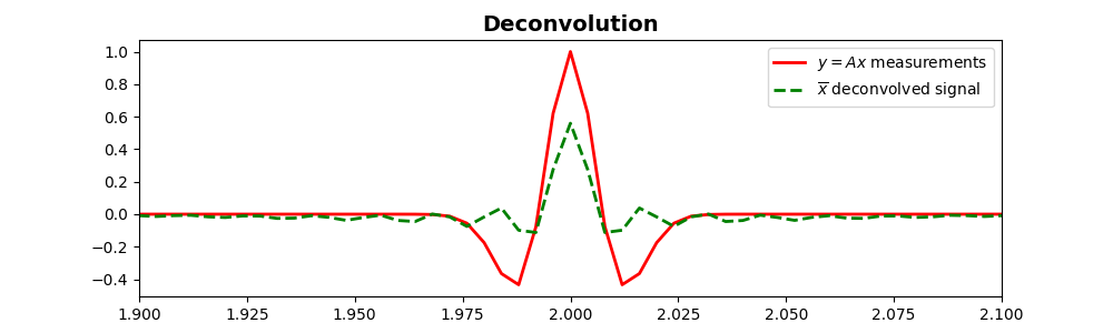
Deconvolution to clean the signal using LSQR
An initial guess of the actual signal is all zeros
x0 = jnp.zeros(n)
# We run LSQR algorithm to clean the signal contents for 25 iterations
sol = sls.lsqr(H, y, x0, max_iters=25)
# Plot the recovered signal against the measured signal
fig, ax = plt.subplots(1, 1, figsize=(10, 3))
ax.plot(t, y, 'r', lw=2, label=r'$y=Ax$ measurements')
ax.plot(t, sol.x, '--g', lw=2, label=r'$\overline{x}$ deconvolved signal')
ax.set_title('Deconvolution', fontsize=14, fontweight='bold')
ax.legend()
# Focus on the middle part
ax.set_xlim(1.9, 2.1)

# Estimated values from the algorithm
print("A norm: ", sol.A_norm)
print("A condition number: ", sol.A_cond)
print("r_norm: ", sol.r_norm, "x_norm: ", sol.x_norm, "atr_norm: ", sol.atr_norm)
print("Iterations: ", sol.iterations, " H x calls: ", sol.n_times, "H^T x calls: ", sol.n_trans)
A norm:  12.19240848747446
A condition number:  59.63129718252214
r_norm:  0.027126481687630485 x_norm:  0.7360252062150451 atr_norm:  0.014044078613519402
Iterations:  25  H x calls:  25 H^T x calls:  25
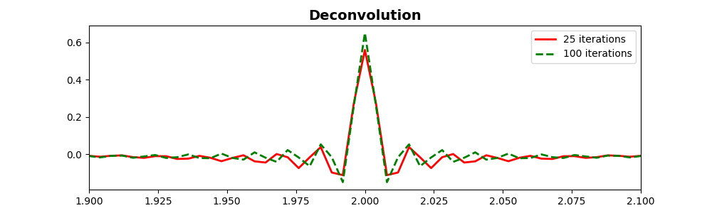
Stronger deconvolution
We run LSQR algorithm to clean the signal contents for 100 iterations
sol2 = sls.lsqr(H, y, x0, max_iters=100)
# Plot the recovered signal against the measured signal
fig, ax = plt.subplots(1, 1, figsize=(10, 3))
ax.plot(t, sol.x, 'r', lw=2, label=r'25 iterations')
ax.plot(t, sol2.x, '--g', lw=2, label=r'100 iterations')
ax.set_title('Deconvolution', fontsize=14, fontweight='bold')
ax.legend()
# Focus on the middle part
ax.set_xlim(1.9, 2.1)

print("A norm: ", sol2.A_norm)
print("A condition number: ", sol2.A_cond)
print("r_norm: ", sol2.r_norm, "x_norm: ", sol2.x_norm, "atr_norm: ", sol2.atr_norm)
print("Iterations: ", sol2.iterations, " H x calls: ", sol2.n_times, "H^T x calls: ", sol2.n_trans)
A norm:  24.348380483410278
A condition number:  485.89437292086
r_norm:  0.005893971270357629 x_norm:  0.7979078081486051 atr_norm:  0.001562908052262193
Iterations:  100  H x calls:  100 H^T x calls:  100
Total running time of the script: (0 minutes 2.312 seconds)
