Note
Go to the end to download the full example code
Wavelet Transform Operators
This example demonstrates following features:
cr.sparse.lop.convolve2DA 2D convolution linear operatorcr.sparse.sls.lsqrLSQR algorithm for solving a least square problem on 2D images
Let’s import necessary libraries
import jax.numpy as jnp
# For plotting diagrams
import matplotlib.pyplot as plt
## CR-Sparse modules
import cr.nimble as cnb
# Linear operators
from cr.sparse import lop
# Sample images
import skimage.data
# Utilities
from cr.nimble.dsp import time_values
# Configure JAX for 64-bit computing
from jax.config import config
config.update("jax_enable_x64", True)
1D Wavelet Transform Operator
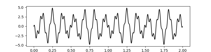
A signal consisting of multiple sinusoids
Individual sinusoids have different frequencies and amplitudes. Sampling frequency
fs = 1000.
# Time duration
T = 2
# time values
t = time_values(fs, T)
# Number of samples
n = t.size
x = jnp.zeros(n)
freqs = [25, 7, 9]
amps = [1, -3, .8]
for  (f, amp) in zip(freqs, amps):
    sinusoid = amp * jnp.sin(2 * jnp.pi * f * t)
    x = x + sinusoid
# Plot the signal
plt.figure(figsize=(8,2))
plt.plot(t, x, 'k', label='Composite signal')
[<matplotlib.lines.Line2D object at 0x7f27b2c2f250>]
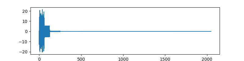
1D wavelet transform operator
DWT_op = lop.dwt(n, wavelet='dmey', level=5)
Wavelet coefficients
alpha = DWT_op.times(x)
plt.figure(figsize=(8,2))
plt.plot(alpha, label='Wavelet coefficients')
[<matplotlib.lines.Line2D object at 0x7f27b09fdd00>]
Compression
Let’s keep only 10 percent of the coefficients
cutoff = n // 10
alpha2 = alpha.at[cutoff:].set(0)
plt.figure(figsize=(8,2))
plt.plot(alpha2, label='Wavelet coefficients after compression')

[<matplotlib.lines.Line2D object at 0x7f27b0176a30>]
Reconstruction
x_rec = DWT_op.trans(alpha2)
# RMSE
rmse = cnb.root_mse(x, x_rec)
print(rmse)
# SNR
snr = cnb.signal_noise_ratio(x, x_rec)
print(snr)
plt.figure(figsize=(8,2))
plt.plot(x, 'k', label='Original')
plt.plot(x_rec, 'r', label='Reconstructed')
plt.title('Reconstructed signal')
plt.legend()
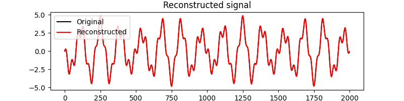
0.034259365997888466
36.56352988951201

<matplotlib.legend.Legend object at 0x7f27b022cfd0>
2D Wavelet Transform Operator
# Sample image
image = skimage.data.grass()
DWT2_op = lop.dwt2D(image.shape, wavelet='haar', level=5)
DWT2_op = lop.jit(DWT2_op)
Wavelet coefficients
coefs = DWT2_op.times(image)
Compression
Let’s keep only 1/16 of the coefficients
Reconstruction
image_rec = DWT2_op.trans(coefs2)
# RMSE
rmse = cnb.root_mse(image, image_rec)
print(rmse)
# PSNR
psnr = cnb.peak_signal_noise_ratio(image, image_rec)
print(psnr)

# Plot everything
fig, axs = plt.subplots(1, 4, figsize=(16, 3))
axs[0].imshow(image, cmap='gray')
axs[0].set_title('Image')
axs[0].axis('tight')

axs[1].imshow(coefs, cmap='gray_r', vmin=-1e2, vmax=1e2)
axs[1].set_title('DWT2 coefficients')
axs[1].axis('tight')

axs[2].imshow(coefs2, cmap='gray_r', vmin=-1e2, vmax=1e2)
axs[2].set_title('After compression')
axs[2].axis('tight')

axs[3].imshow(image_rec, cmap='gray')
axs[3].set_title('Reconstructed image')
axs[3].axis('tight')
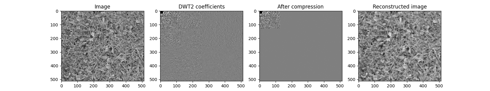
27.383743287757877
19.380947312633058

(-0.5, 511.5, 511.5, -0.5)
Total running time of the script: (0 minutes 4.833 seconds)
