Note
Go to the end to download the full example code
1 bit Compressive Sensing
This example demonstrates following features - Making 1-bit quantized compressive measurements of a sparse signal - Recovering the original signal using the BIHT (Binary Iterative Hard Thresholding) algorithm.
Let’s import necessary libraries
import jax.numpy as jnp
from jax.numpy.linalg import norm

import matplotlib as mpl
import matplotlib.pyplot as plt

import cr.nimble as cnb
import cr.sparse as crs
import cr.sparse.dict as crdict
import cr.sparse.data as crdata
import cr.sparse.cs.cs1bit as cs1bit

from cr.nimble.dsp import (
    build_signal_from_indices_and_values
)
Setup
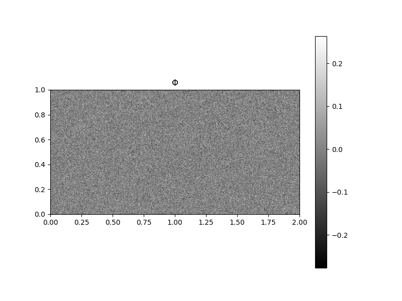
Sensing Matrix
Phi = crdict.gaussian_mtx(cnb.KEYS[0], M, N, normalize_atoms=False)
# frame bound
s0 = crdict.upper_frame_bound(Phi)
print(s0)
fig=plt.figure(figsize=(8,6), dpi= 100, facecolor='w', edgecolor='k')
plt.imshow(Phi, extent=[0, 2, 0, 1])
plt.gray()
plt.colorbar()
plt.title(r'$\Phi$')
2.4003416483791433

Text(0.5, 1.0, '$\\Phi$')
K-sparse signal
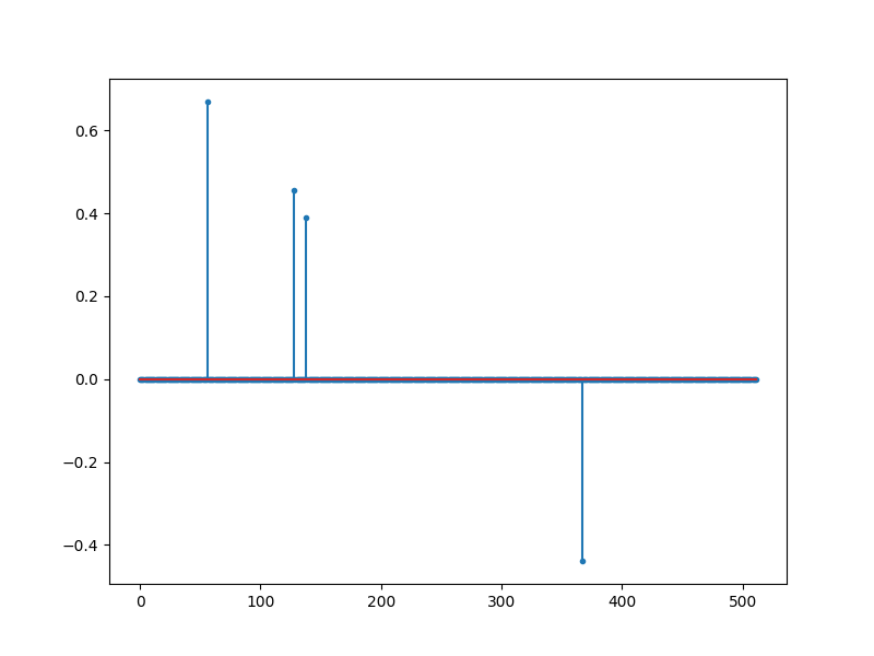
[ 56 128 138 367]

<StemContainer object of 3 artists>
Measurement process
measurements
y = cs1bit.measure_1bit(Phi, x)
fig=plt.figure(figsize=(8,6), dpi= 100, facecolor='w', edgecolor='k')
plt.stem(y, markerfmt='.')
print(y)
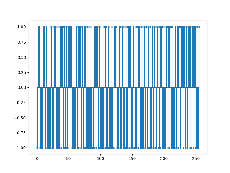
[-1. -1.  1.  1.  1. -1. -1. -1. -1. -1.  1.  1.  1. -1. -1.  1. -1. -1.
 -1. -1. -1. -1.  1.  1. -1. -1. -1.  1.  1.  1.  1. -1. -1.  1. -1. -1.
  1.  1. -1.  1.  1.  1. -1. -1.  1. -1. -1.  1. -1. -1.  1.  1.  1.  1.
  1. -1. -1. -1. -1. -1. -1. -1.  1.  1. -1. -1.  1.  1. -1.  1. -1.  1.
  1. -1. -1.  1. -1.  1. -1.  1. -1. -1.  1. -1. -1.  1. -1. -1. -1. -1.
 -1.  1.  1. -1.  1.  1.  1. -1. -1.  1. -1. -1. -1. -1. -1. -1.  1. -1.
  1.  1. -1. -1. -1.  1. -1. -1. -1. -1.  1. -1. -1. -1.  1.  1.  1.  1.
 -1. -1. -1. -1.  1.  1. -1. -1.  1.  1. -1.  1. -1. -1.  1. -1.  1. -1.
  1. -1.  1.  1. -1. -1. -1. -1.  1. -1. -1. -1.  1. -1.  1. -1.  1.  1.
  1. -1.  1. -1. -1.  1. -1.  1.  1. -1.  1.  1. -1. -1.  1. -1.  1. -1.
 -1. -1.  1. -1.  1.  1. -1.  1. -1.  1.  1. -1.  1. -1. -1.  1.  1.  1.
 -1. -1.  1. -1. -1.  1.  1.  1. -1.  1. -1.  1.  1.  1. -1.  1. -1. -1.
 -1. -1.  1. -1. -1.  1. -1.  1.  1.  1. -1.  1.  1.  1. -1.  1.  1.  1.
 -1.  1. -1. -1.  1.  1.  1. -1.  1. -1.  1.  1. -1.  1.  1. -1.  1. -1.
  1. -1. -1.  1.]
Signal Reconstruction using BIHT
solver step-size
tau = 0.98 * s0
# solution
sol = cs1bit.biht_jit(Phi, y, K, tau)
reconstructed signal
x_rec = build_signal_from_indices_and_values(N, sol.I, sol.x_I)
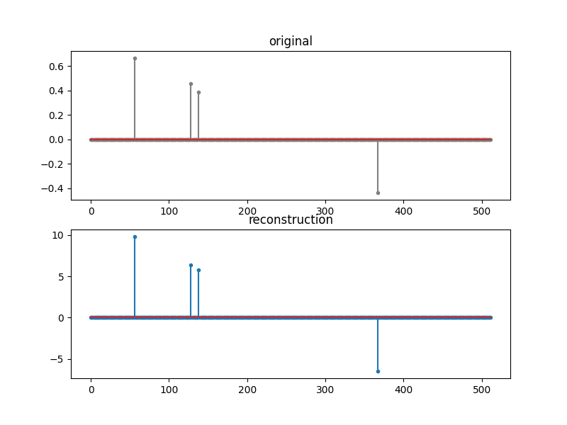
Verification
fig=plt.figure(figsize=(8,6), dpi= 100, facecolor='w', edgecolor='k')
plt.subplot(211)
plt.title('original')
plt.stem(x, markerfmt='.', linefmt='gray')
plt.subplot(212)
plt.stem(x_rec, markerfmt='.')
plt.title('reconstruction')

# recovered support
I = jnp.sort(sol.I)
print(I)
[ 56 128 138 367]
check if the support is recovered correctly
print(jnp.array_equal(omega, I))
# normalize recovered signal
x_rec = x_rec / norm(x_rec)
# the norm of error
print(norm(x - x_rec))
True
0.024352999672904573
Total running time of the script: (0 minutes 1.923 seconds)
