CoSaMP step by step

This example explains the step by step development of CoSaMP (Compressive Sensing Matching Pursuit) algorithm for sparse recovery. It then shows how to use the official implementation of CoSaMP in CR-Sparse.

The CoSaMP algorithm has following inputs:

• A sensing matrix or dictionary Phi which has been used for data measurements.

• A measurement vector y.

• The sparsity level K.

The objective of the algorithm is to estimate a K-sparse solution x such that y is approximately equal to Phi x.

A key quantity in the algorithm is the residual r = y - Phi x. Each iteration of the algorithm successively improves the estimate x so that the energy of the residual r reduces.

The algorithm proceeds as follows:

• Initialize the solution x with zero.

• Maintain an index set I (initially empty) of atoms selected as part of the solution.

• While the residual energy is above a threshold:

• Match: Compute the inner product of each atom in Phi with the current residual r.

• Identify: Select the indices of 2K atoms from Phi with the largest correlation with the residual.

• Merge: merge these 2K indices with currently selected indices in I to form I_sub.

• LS: Compute the least squares solution of Phi[:, I_sub] z = y

• Prune: Pick the largest K entries from this least square solution and keep them in I.

• Update residual: Compute r = y - Phi_I x_I.

It is time to see the algorithm in action.

Let’s import necessary libraries

import jax
from jax import random
import jax.numpy as jnp
# Some keys for generating random numbers
key = random.PRNGKey(0)
keys = random.split(key, 4)

# For plotting diagrams
import matplotlib.pyplot as plt
# CR-Sparse modules
import cr.sparse as crs
import cr.sparse.dict as crdict
import cr.sparse.data as crdata
from cr.nimble.dsp import (
    nonzero_indices,
    nonzero_values,
    largest_indices
)

Problem Setup

# Number of measurements
M = 128
# Ambient dimension
N = 256
# Sparsity level
K = 8

The Sparsifying Basis

Phi = crdict.gaussian_mtx(key, M,N)
print(Phi.shape)

(128, 256)

Coherence of atoms in the sensing matrix

print(crdict.coherence(Phi))

0.3881940752728321

A sparse model vector

x0, omega = crdata.sparse_normal_representations(key, N, K)
plt.figure(figsize=(8,6), dpi= 100, facecolor='w', edgecolor='k')
plt.plot(x0)

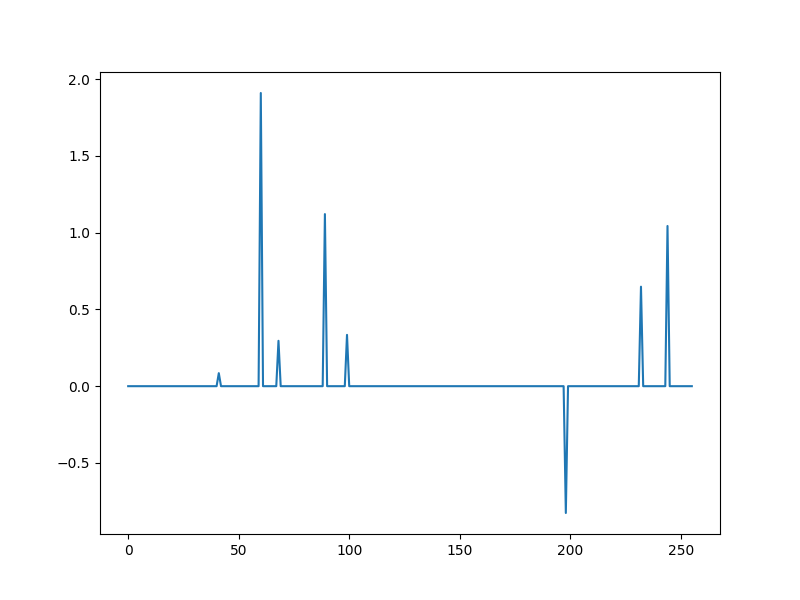
[<matplotlib.lines.Line2D object at 0x7f27b03ea1f0>]

omega contains the set of indices at which x is nonzero (support of x)

print(omega)

[ 41  60  68  89  99 198 232 244]

Compressive measurements

y = Phi @ x0
plt.figure(figsize=(8,6), dpi= 100, facecolor='w', edgecolor='k')
plt.plot(y)

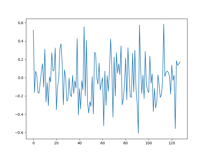
[<matplotlib.lines.Line2D object at 0x7f27ac2a8e80>]

Development of CoSaMP algorithm

# In the following, we walk through the steps of CoSaMP algorithm.
# Since we have access to ``x0`` and ``omega``, we can measure the
# progress made by the algorithm steps by comparing the estimates
# with actual ``x0`` and ``omega``. However, note that in the
# real implementation of the algorithm, no access to original model
# vector is there.
#
# Initialization
# ''''''''''''''''''''''''''''''''''''''''''''

We assume the initial solution to be zero and the residual r = y - Phi x to equal the measurements y

r = y

Squared norm/energy of the residual

y_norm_sqr = float(y.T @ y)
r_norm_sqr = y_norm_sqr
print(f"{r_norm_sqr=}")

r_norm_sqr=7.401212029141624

A boolean array to track the indices selected for least squares steps

flags = jnp.zeros(N, dtype=bool)

During the matching steps, 2K atoms will be picked.

K2 = 2*K

At any time, up to 3K atoms may be selected (after the merge step).

K3 = K + K2

Number of iterations completed so far

iterations = 0

A limit on the maximum tolerance for residual norm

res_norm_rtol = 1e-3
max_r_norm_sqr = y_norm_sqr * (res_norm_rtol ** 2)
print(f"{max_r_norm_sqr=:.2e}")

max_r_norm_sqr=7.40e-06

First iteration

print("First iteration:")

First iteration:

Match the current residual with the atoms in Phi

h = Phi.T @ r

Pick the indices of 3K atoms with largest matches with the residual

I_sub =  largest_indices(h, K3)
# Update the flags array
flags = flags.at[I_sub].set(True)
# Sort the ``I_sub`` array with the help of flags array
I_sub, = jnp.where(flags)
# Since no atoms have been selected so far, we can be more aggressive
# and pick 3K atoms in first iteration.
print(f"{I_sub=}")

I_sub=Array([ 14,  30,  44,  60,  64,  78,  84,  89,  99, 116, 118, 127, 128,
       149, 157, 158, 162, 168, 184, 192, 198, 203, 232, 244],      dtype=int64)

Check which indices from omega are there in I_sub.

print(jnp.intersect1d(omega, I_sub))

[ 60  89  99 198 232 244]

Select the subdictionary of Phi consisting of atoms indexed by I_sub

Phi_sub = Phi[:, flags]

Compute the least squares solution of y over this subdictionary

x_sub, r_sub_norms, rank_sub, s_sub = jnp.linalg.lstsq(Phi_sub, y)
# Pick the indices of K largest entries in in ``x_sub``
Ia = largest_indices(x_sub, K)
print(f"{Ia=}")

Ia=Array([ 3,  7, 23, 20, 22,  8, 15, 18], dtype=int64)

We need to map the indices in Ia to the actual indices of atoms in Phi

I = I_sub[Ia]
print(f"{I=}")

I=Array([ 60,  89, 244, 198, 232,  99, 158, 184], dtype=int64)

Select the corresponding values from the LS solution

x_I = x_sub[Ia]

We now have our first estimate of the solution

x = jnp.zeros(N).at[I].set(x_I)
plt.figure(figsize=(8,6), dpi= 100, facecolor='w', edgecolor='k')
plt.plot(x0, label="Original vector")
plt.plot(x, '--', label="Estimated solution")
plt.legend()

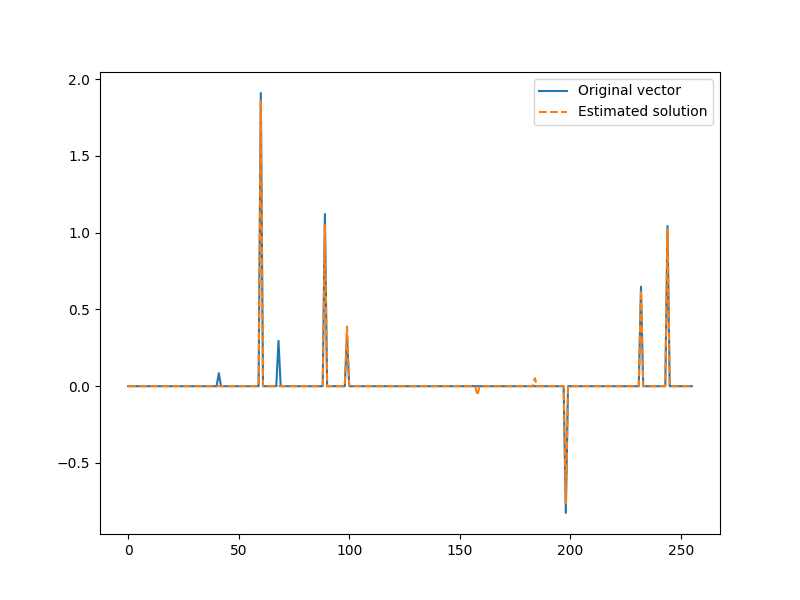
<matplotlib.legend.Legend object at 0x7f27abe7e790>

We can check how good we were in picking the correct indices from the actual support of the signal

found = jnp.intersect1d(omega, I)
print("Found indices: ", found)

Found indices:  [ 60  89  99 198 232 244]

We found 6 out of 8 indices in the support. Here are the remaining.

missing = jnp.setdiff1d(omega, I)
print("Missing indices: ", missing)

Missing indices:  [41 68]

It is time to compute the residual after the first iteration

Phi_I = Phi[:, I]
r = y - Phi_I @ x_I

Compute the residual and verify that it is still larger than the allowed tolerance

r_norm_sqr = float(r.T @ r)
print(f"{r_norm_sqr=:.2e} > {max_r_norm_sqr=:.2e}")

r_norm_sqr=8.28e-02 > max_r_norm_sqr=7.40e-06

Store the selected K indices in the flags array

flags = flags.at[:].set(False)
flags = flags.at[I].set(True)
print(jnp.where(flags))

(Array([ 60,  89,  99, 158, 184, 198, 232, 244], dtype=int64),)

Mark the completion of the iteration

iterations += 1

Second iteration

print("Second iteration:")

Second iteration:

Match the current residual with the atoms in Phi

h = Phi.T @ r

Pick the indices of 2K atoms with largest matches with the residual

I_2k =  largest_indices(h, K2 if iterations else K3)
# We can check if these include the atoms missed out in first iteration.
print(jnp.intersect1d(omega, I_2k))

[41 68]

Merge (union) the set of previous K indices with the new 2K indices

flags = flags.at[I_2k].set(True)
I_sub, = jnp.where(flags)
print(f"{I_sub=}")

I_sub=Array([  8,  25,  41,  42,  60,  66,  67,  68,  72,  89,  99, 111, 129,
       158, 164, 184, 190, 195, 198, 216, 220, 232, 233, 244],      dtype=int64)

We can check if we found all the actual atoms

print("Found in I_sub: ", jnp.intersect1d(omega, I_sub))

Found in I_sub:  [ 41  60  68  89  99 198 232 244]

Indeed we did. The set difference is empty.

print("Missing in I_sub: ", jnp.setdiff1d(omega, I_sub))

Missing in I_sub:  []

Select the subdictionary of Phi consisting of atoms indexed by I_sub

Phi_sub = Phi[:, flags]

Compute the least squares solution of y over this subdictionary

x_sub, r_sub_norms, rank_sub, s_sub = jnp.linalg.lstsq(Phi_sub, y)
# Pick the indices of K largest entries in in ``x_sub``
Ia = largest_indices(x_sub, K)
print(Ia)

[ 4  9 23 18 21 10  7  2]

We need to map the indices in Ia to the actual indices of atoms in Phi

I = I_sub[Ia]
print(I)

[ 60  89 244 198 232  99  68  41]

Check if the final K indices in I include all the indices in omega

jnp.setdiff1d(omega, I)

Array([], dtype=int64)

Select the corresponding values from the LS solution

x_I = x_sub[Ia]

Here is our updated estimate of the solution

x = jnp.zeros(N).at[I].set(x_I)
plt.figure(figsize=(8,6), dpi= 100, facecolor='w', edgecolor='k')
plt.plot(x0, label="Original vector")
plt.plot(x, '--', label="Estimated solution")
plt.legend()

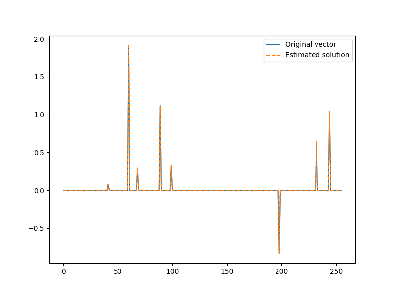
<matplotlib.legend.Legend object at 0x7f27aca73910>

The algorithm has no direct way of knowing that it indeed found the solution It is time to compute the residual after the second iteration

Phi_I = Phi[:, I]
r = y - Phi_I @ x_I

Compute the residual and verify that it is now below the allowed tolerance

r_norm_sqr = float(r.T @ r)
# It turns out that it is now below the tolerance threshold
print(f"{r_norm_sqr=:.2e} < {max_r_norm_sqr=:.2e}")

r_norm_sqr=7.09e-30 < max_r_norm_sqr=7.40e-06

We have completed the signal recovery. We can stop iterating now.

iterations += 1

CR-Sparse official implementation

The JIT compiled version of this algorithm is available in cr.sparse.pursuit.cosamp module.

Import the module

from cr.sparse.pursuit import cosamp

Run the solver

solution =  cosamp.matrix_solve_jit(Phi, y, K)
# The support for the sparse solution
I = solution.I
print(I)

[ 60  89 244 198 232  99  68  41]

The non-zero values on the support

x_I = solution.x_I
print(x_I)

[ 1.9097652   1.12094818  1.04348768 -0.82606793  0.64812788  0.33432345
  0.29561749  0.08482584]

Verify that we successfully recovered the support

print(jnp.setdiff1d(omega, I))

[]

Print the residual energy and the number of iterations when the algorithm converged.

print(solution.r_norm_sqr, solution.iterations)

7.726387804898689e-30 3

Let’s plot the solution

x = jnp.zeros(N).at[I].set(x_I)
plt.figure(figsize=(8,6), dpi= 100, facecolor='w', edgecolor='k')
plt.plot(x0, label="Original vector")
plt.plot(x, '--', label="Estimated solution")
plt.legend()

<matplotlib.legend.Legend object at 0x7f27ac4d59d0>