ECG Data Compressive Sensing

In this example, we demonstrate the compressive sensing of ECG data and reconstruction using Block Sparse Bayesian Learning (BSBL).

# Configure JAX to work with 64-bit floating point precision.
from jax.config import config
config.update("jax_enable_x64", True)

Let’s import necessary libraries

import timeit
import jax
import numpy as np
import jax.numpy as jnp
# CR-Suite libraries
import cr.nimble as crn
import cr.nimble.dsp as crdsp
import cr.sparse.dict as crdict
import cr.sparse.plots as crplot
import cr.sparse.block.bsbl as bsbl

# Sample data
from scipy.misc import electrocardiogram
# Plotting
import matplotlib.pyplot as plt
# Miscellaneous
from scipy.signal import detrend, butter, filtfilt

Test signal

SciPy includes a test electrocardiogram signal which is a 5 minute long electrocardiogram (ECG), a medical recording of the electrical activity of the heart, sampled at 360 Hz.

ecg = electrocardiogram()
# Sampling frequency in Hz
fs = 360
# We shall only process a part of the signal in this demo
N = 400
x = ecg[:N]
t = np.arange(N) * (1/fs)
fig, ax = plt.subplots(figsize=(16,4))
ax.plot(t, x);

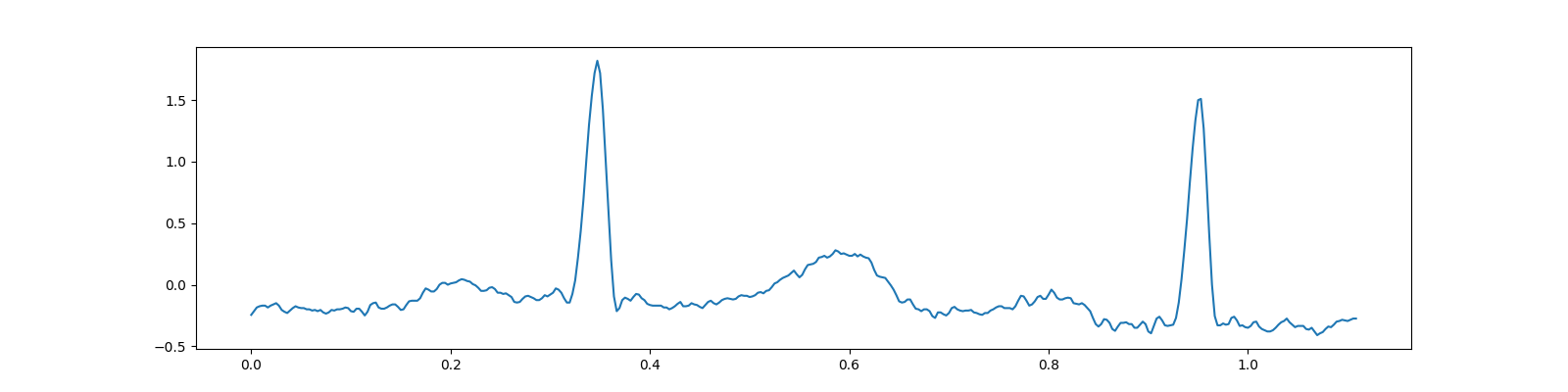
/home/docs/checkouts/readthedocs.org/user_builds/cr-sparse/checkouts/latest/examples/0200_cs/ecg_cs_bsbl.py:48: DeprecationWarning: scipy.misc.electrocardiogram has been deprecated in SciPy v1.10.0; and will be completely removed in SciPy v1.12.0. Dataset methods have moved into the scipy.datasets module. Use scipy.datasets.electrocardiogram instead.
  ecg = electrocardiogram()

[<matplotlib.lines.Line2D object at 0x7f27ac6e4190>]

Preprocessing

# Remove the linear trend from the signal
x = detrend(x)
## bandpass filter
# lower cutoff frequency
f1 = 5
# upper cutoff frequency
f2 = 40
# passband in normalized frequency
Wn = np.array([f1, f2]) * 2 / fs
# butterworth filter
fn = 3
fb, fa = butter(fn, Wn, 'bandpass')
x = filtfilt(fb,fa,x)
fig, ax = plt.subplots(figsize=(16,4))
ax.plot(t, x);

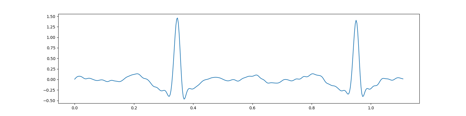
[<matplotlib.lines.Line2D object at 0x7f27ac6814f0>]

Compressive Sensing at 70%

We choose the compression ratio (M/N) to be 0.7

CR = 0.70
M = int(N * CR)
print(f'M={M}, N={N}, CR={CR}')

M=280, N=400, CR=0.7

Sensing matrix

Phi = crdict.gaussian_mtx(crn.KEY0, M, N)

Measurements

y = Phi @ x
fig, ax = plt.subplots(figsize=(16, 4))
ax.plot(y);

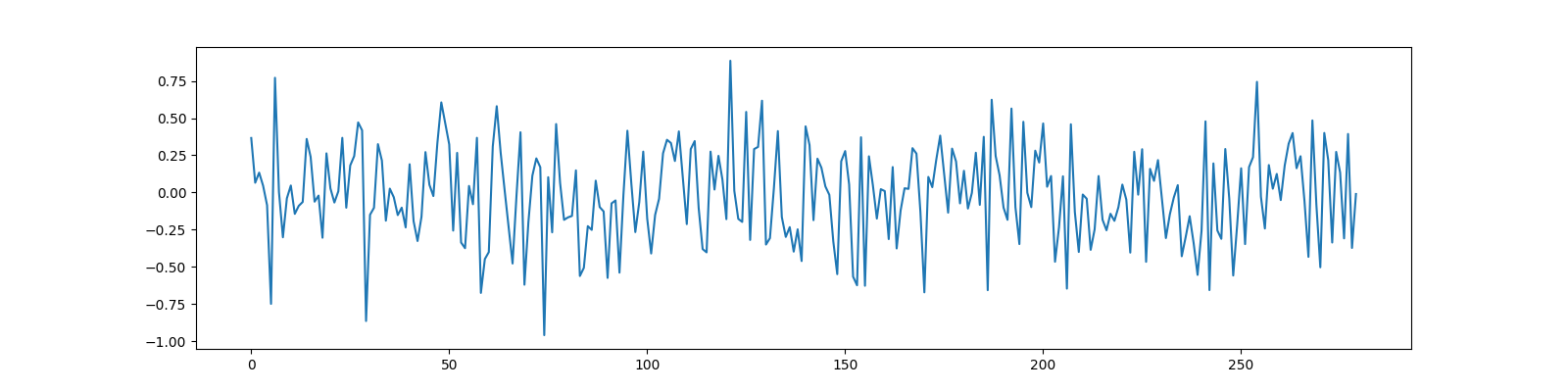
[<matplotlib.lines.Line2D object at 0x7f27ac0d6a30>]

Sparse Recovery with BSBL

options = bsbl.bsbl_bo_options(y, max_iters=20)
start = timeit.default_timer()
sol = bsbl.bsbl_bo_np_jit(Phi, y, 25, options=options)
stop = timeit.default_timer()
print(f'Reconstruction time: {stop - start:.2f} sec', )
print(sol)

Reconstruction time: 1.70 sec
iterations=20
block size=25
blocks=16, nonzero=16
r_norm=1.49e-01
x_norm=5.23e+00
lambda=5.86e-04
dmu=1.49e-04

Recovered signal

x_hat = sol.x
print(f'SNR: {crn.signal_noise_ratio(x, x_hat):.2f} dB, PRD: {crn.percent_rms_diff(x, x_hat):.1f}%')

SNR: 24.79 dB, PRD: 5.8%

Plot the original and recovered signals

ax = crplot.h_plots(2)
ax[0].plot(x)
ax[1].plot(x_hat)

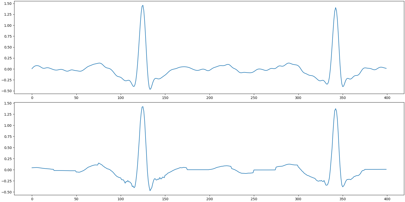
[<matplotlib.lines.Line2D object at 0x7f27ac14d490>]

Compressive Sensing at 50%

Let us now increase the compression

CR = 0.50
M = int(N * CR)
print(f'M={M}, N={N}, CR={CR}')

M=200, N=400, CR=0.5

Sensing matrix

Phi = crdict.gaussian_mtx(crn.KEY0, M, N)

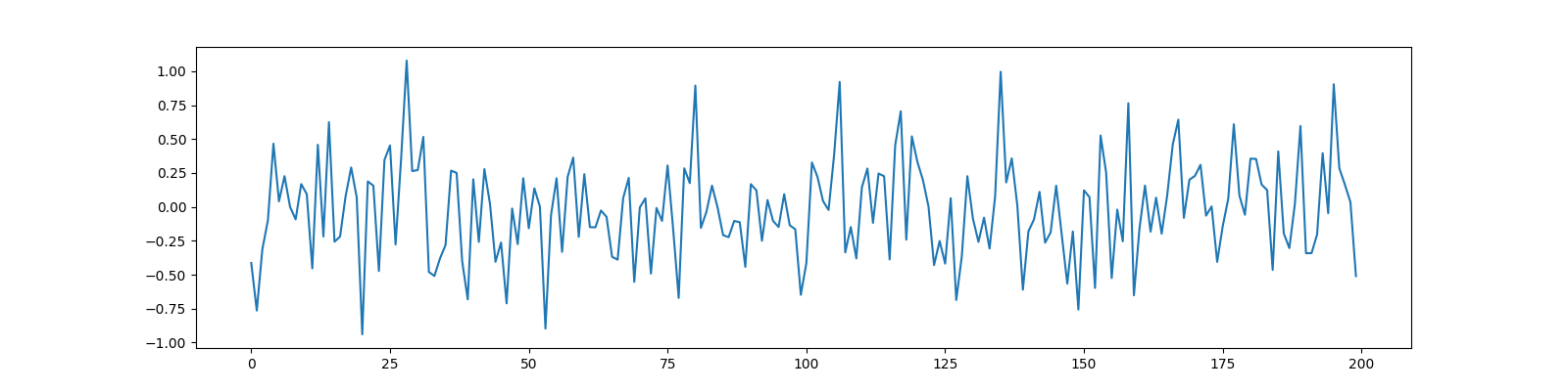
Measurements

y = Phi @ x
fig, ax = plt.subplots(figsize=(16, 4))
ax.plot(y);

[<matplotlib.lines.Line2D object at 0x7f27ac772670>]

Sparse Recovery with BSBL

options = bsbl.bsbl_bo_options(y, max_iters=20)
start = timeit.default_timer()
sol = bsbl.bsbl_bo_np_jit(Phi, y, 25, options=options)
stop = timeit.default_timer()
print(f'Reconstruction time: {stop - start:.2f} sec', )
print(sol)

Reconstruction time: 1.38 sec
iterations=20
block size=25
blocks=16, nonzero=16
r_norm=2.43e-01
x_norm=5.13e+00
lambda=2.20e-03
dmu=2.36e-03

Recovered signal

x_hat = sol.x
print(f'SNR: {crn.signal_noise_ratio(x, x_hat):.2f} dB, PRD: {crn.percent_rms_diff(x, x_hat):.1f}%')

SNR: 20.33 dB, PRD: 9.6%

Plot the original and recovered signals

ax = crplot.h_plots(2)
ax[0].plot(x)
ax[1].plot(x_hat)

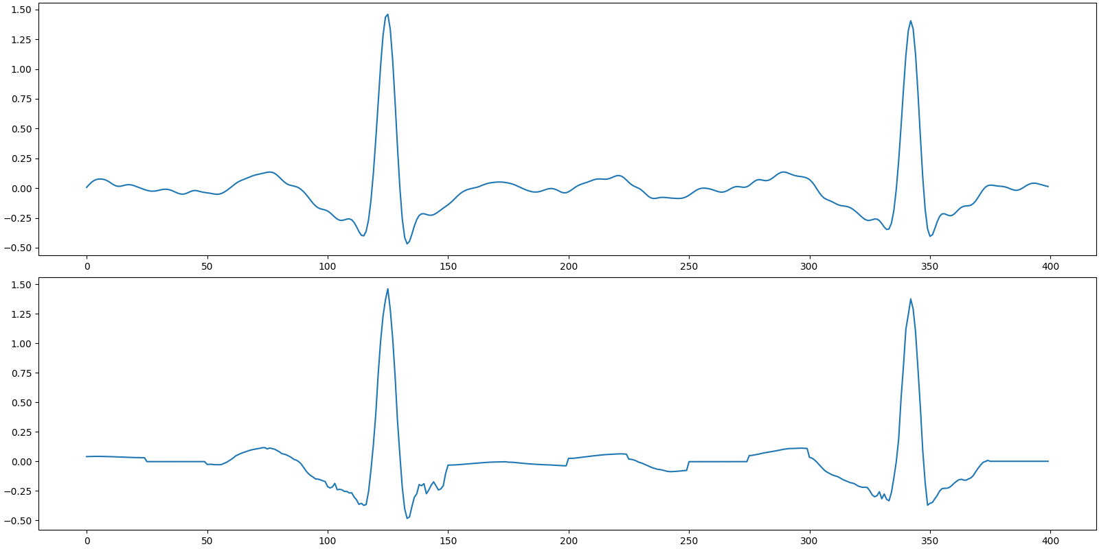
[<matplotlib.lines.Line2D object at 0x7f27ac2165b0>]