Note

Go to the end to download the full example code

Sparse Binary Sensing Matrices¶

Creating Sparse Binary Sensing Matrices
Sparse Binary Sensing Linear Operators
Compressive Sensing
Sparse Recovery

A (random) sparse binary sensing matrix has a very simple design. Assume that the signal space is \(\RR^N\) and the measurement space is \(\RR^M\). Every column of a sparse binary sensing matrix has a 1 in exactly \(d\) positions and 0s elsewhere. The indices at which ones are present are randomly selected for each column.

Following is an example sparse binary matrix with 3 ones in each column

(1)¶\[\begin{split}\begin{bmatrix} 1 & 0 & 0 & 0 & 0 & 0 & 1 & 1 & 0 & 0 & 1 & 0 & 0 & 0 & 0 & 1\\ 0 & 0 & 0 & 0 & 0 & 1 & 0 & 0 & 0 & 1 & 1 & 1 & 0 & 1 & 0 & 0\\ 0 & 0 & 0 & 1 & 1 & 1 & 0 & 0 & 1 & 0 & 0 & 0 & 0 & 1 & 0 & 0\\ 0 & 1 & 0 & 0 & 0 & 0 & 0 & 0 & 0 & 1 & 0 & 0 & 0 & 0 & 0 & 0\\ 0 & 0 & 0 & 1 & 0 & 0 & 0 & 1 & 0 & 0 & 0 & 0 & 1 & 0 & 0 & 0\\ 0 & 1 & 0 & 0 & 0 & 0 & 0 & 0 & 1 & 0 & 1 & 0 & 1 & 0 & 1 & 1\\ 1 & 0 & 0 & 1 & 1 & 0 & 0 & 0 & 0 & 0 & 0 & 1 & 0 & 0 & 1 & 0\\ 1 & 0 & 1 & 0 & 0 & 1 & 1 & 1 & 0 & 0 & 0 & 1 & 0 & 0 & 1 & 0\\ 0 & 1 & 1 & 0 & 1 & 0 & 0 & 0 & 1 & 1 & 0 & 0 & 0 & 1 & 0 & 1\\ 0 & 0 & 1 & 0 & 0 & 0 & 1 & 0 & 0 & 0 & 0 & 0 & 1 & 0 & 0 & 0\\ \end{bmatrix}\end{split}\]

From the perspective of algorithm design, we often require that the sensing matrix have unit norm columns. This can be easily attained for sparse binary matrices by scaling them with \(\frac{1}{\sqrt{d}}\).

JAX provides an efficient way of storing sparse matrices in BCOO format. By default we employ this storage format for the (random) sparse binary matrices.

Necessary imports

import math
import cr.nimble as crn
import cr.sparse as crs
import cr.sparse.dict as crdict
import cr.sparse.data as crdata
import cr.sparse.lop as crlop
import cr.sparse.plots as crplots
import numpy as np
import jax
import jax.numpy as jnp
from jax import random

Some random number generation keys

key = random.PRNGKey(3)
keys = random.split(key, 5)

Creating Sparse Binary Sensing Matrices ¶

# Matrix parameters
m = 10
n = 16
d = 4

# construct a sparse binary sensing matrix
A = crdict.sparse_binary_mtx(keys[0], m, n, d, normalize_atoms=False)
# It is stored in a compressed BCOO format
print(A)

BCOO(uint8[10, 16], nse=64)

If we wish to see its contents

Ad = A.todense()
print(Ad)

[[0 0 0 1 1 0 0 1 1 0 0 1 1 1 1 0]
 [1 0 1 0 0 1 1 1 0 1 0 0 1 0 1 0]
 [0 0 0 0 0 0 0 0 1 0 0 1 0 0 0 1]
 [1 1 0 0 1 0 0 1 0 0 1 0 1 0 0 0]
 [1 1 1 0 1 1 0 0 1 1 1 0 0 0 0 0]
 [0 1 0 1 0 0 0 0 0 0 0 0 0 0 0 1]
 [0 0 0 1 0 0 0 0 0 0 0 0 0 0 1 0]
 [0 1 1 0 0 1 1 0 0 1 1 1 1 1 1 1]
 [0 0 0 1 1 1 1 1 1 0 0 0 0 1 0 1]
 [1 0 1 0 0 0 1 0 0 1 1 1 0 1 0 0]]

We can quickly check that all columns have d ones

print(jnp.sum(Ad, 0))

[4 4 4 4 4 4 4 4 4 4 4 4 4 4 4 4]

By convention, we generate normalized sensing matrices by default. However, in the case of sparse binary matrices, it is more efficient to work with the unnormalized sensing matrix

A = crdict.sparse_binary_mtx(keys[0], m, n, d)
print(A.todense())

[[0.  0.  0.  0.5 0.5 0.  0.  0.5 0.5 0.  0.  0.5 0.5 0.5 0.5 0. ]
 [0.5 0.  0.5 0.  0.  0.5 0.5 0.5 0.  0.5 0.  0.  0.5 0.  0.5 0. ]
 [0.  0.  0.  0.  0.  0.  0.  0.  0.5 0.  0.  0.5 0.  0.  0.  0.5]
 [0.5 0.5 0.  0.  0.5 0.  0.  0.5 0.  0.  0.5 0.  0.5 0.  0.  0. ]
 [0.5 0.5 0.5 0.  0.5 0.5 0.  0.  0.5 0.5 0.5 0.  0.  0.  0.  0. ]
 [0.  0.5 0.  0.5 0.  0.  0.  0.  0.  0.  0.  0.  0.  0.  0.  0.5]
 [0.  0.  0.  0.5 0.  0.  0.  0.  0.  0.  0.  0.  0.  0.  0.5 0. ]
 [0.  0.5 0.5 0.  0.  0.5 0.5 0.  0.  0.5 0.5 0.5 0.5 0.5 0.5 0.5]
 [0.  0.  0.  0.5 0.5 0.5 0.5 0.5 0.5 0.  0.  0.  0.  0.5 0.  0.5]
 [0.5 0.  0.5 0.  0.  0.  0.5 0.  0.  0.5 0.5 0.5 0.  0.5 0.  0. ]]

Sparse Binary Sensing Linear Operators ¶

It is often advantageous to work with matrices wrapped in our linear operator design. Let us construct the sensing matrix as a linear operator

T = crlop.sparse_binary_dict(keys[0], m, n, d, normalize_atoms=False)

We can extract the contents by multiplying with an identity matrix

print(T.times(jnp.eye(n, dtype=int)))

[[0 0 0 1 1 0 0 1 1 0 0 1 1 1 1 0]
 [1 0 1 0 0 1 1 1 0 1 0 0 1 0 1 0]
 [0 0 0 0 0 0 0 0 1 0 0 1 0 0 0 1]
 [1 1 0 0 1 0 0 1 0 0 1 0 1 0 0 0]
 [1 1 1 0 1 1 0 0 1 1 1 0 0 0 0 0]
 [0 1 0 1 0 0 0 0 0 0 0 0 0 0 0 1]
 [0 0 0 1 0 0 0 0 0 0 0 0 0 0 1 0]
 [0 1 1 0 0 1 1 0 0 1 1 1 1 1 1 1]
 [0 0 0 1 1 1 1 1 1 0 0 0 0 1 0 1]
 [1 0 1 0 0 0 1 0 0 1 1 1 0 1 0 0]]

We can keep the normalization of the sensing matrix has a separate scaling operator

# Let us construct a scaling operator
d_scale = 1/ math.sqrt(d)
T_scale = crlop.scalar_mult(d_scale, m)
# Let us combine the scaling operator with the unnormalized sensing operator
T_normed = crlop.compose(T_scale, T)
# Verify the normalized operator
print(T_normed.times(jnp.eye(n, dtype=int)))

[[0.  0.  0.  0.5 0.5 0.  0.  0.5 0.5 0.  0.  0.5 0.5 0.5 0.5 0. ]
 [0.5 0.  0.5 0.  0.  0.5 0.5 0.5 0.  0.5 0.  0.  0.5 0.  0.5 0. ]
 [0.  0.  0.  0.  0.  0.  0.  0.  0.5 0.  0.  0.5 0.  0.  0.  0.5]
 [0.5 0.5 0.  0.  0.5 0.  0.  0.5 0.  0.  0.5 0.  0.5 0.  0.  0. ]
 [0.5 0.5 0.5 0.  0.5 0.5 0.  0.  0.5 0.5 0.5 0.  0.  0.  0.  0. ]
 [0.  0.5 0.  0.5 0.  0.  0.  0.  0.  0.  0.  0.  0.  0.  0.  0.5]
 [0.  0.  0.  0.5 0.  0.  0.  0.  0.  0.  0.  0.  0.  0.  0.5 0. ]
 [0.  0.5 0.5 0.  0.  0.5 0.5 0.  0.  0.5 0.5 0.5 0.5 0.5 0.5 0.5]
 [0.  0.  0.  0.5 0.5 0.5 0.5 0.5 0.5 0.  0.  0.  0.  0.5 0.  0.5]
 [0.5 0.  0.5 0.  0.  0.  0.5 0.  0.  0.5 0.5 0.5 0.  0.5 0.  0. ]]

Compressive Sensing ¶

We shall use a larger problem to demonstrate the sensing capabilities of the sparse binary sensing operator.

# Signal space dimension
n = 1024
# Measurement space dimension
m = 256
# Number of ones in each column
d = 16
# Sparsity level of the signal to be sensed
k = 40

Let us construct the unnormalized as well as normalized sensing operators. We shall use the unnormalized one during sensing but the normalized one during reconstruction.

d_scale = 1/ math.sqrt(d)
T = crlop.sparse_binary_dict(keys[1], m, n, d, normalize_atoms=False)
T_scale = crlop.scalar_mult(d_scale, m)
T_normed = crlop.compose(T_scale, T)

We can quickly visualize the sparsity pattern of this sensing matrix

A = T.times(jnp.eye(n, dtype=int))
ax = crplots.one_plot()
ax.spy(A);

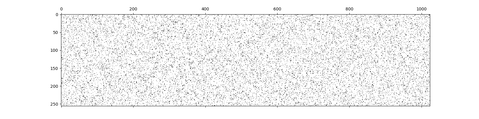
<matplotlib.image.AxesImage object at 0x7f27abd4d610>

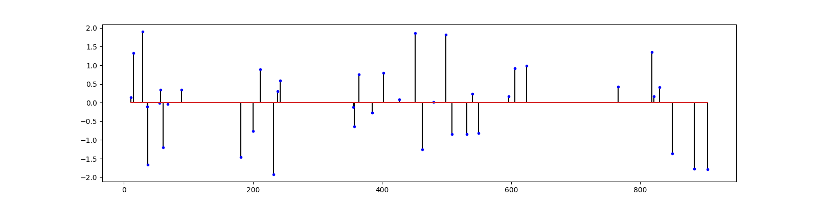
Let us construct a sparse signal

x, omega = crdata.sparse_normal_representations(keys[2], n, k)
ax = crplots.one_plot()
crplots.plot_sparse_signal(ax, x)

y = T.times(x)
ax = crplots.one_plot()
crplots.plot_sparse_signal(ax, y)

Sparse Recovery ¶

We shall use various algorithms for reconstructing the original signal

CoSaMP ¶

# Import the algorithm
from cr.sparse.pursuit import cosamp
# Solve the problem
sol =  cosamp.operator_solve_jit(T_normed, y, k)
print(sol)
# We need to scale the solution since the measurements were unscaled
x_hat = sol.x * d_scale
# Compute the SNR and PRD
print(f'SNR: {crn.signal_noise_ratio(x, x_hat):.2f} dB, PRD: {crn.percent_rms_diff(x, x_hat):.0f} %')
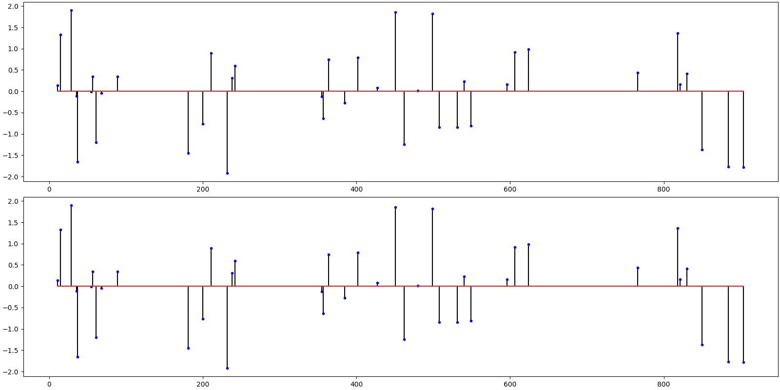
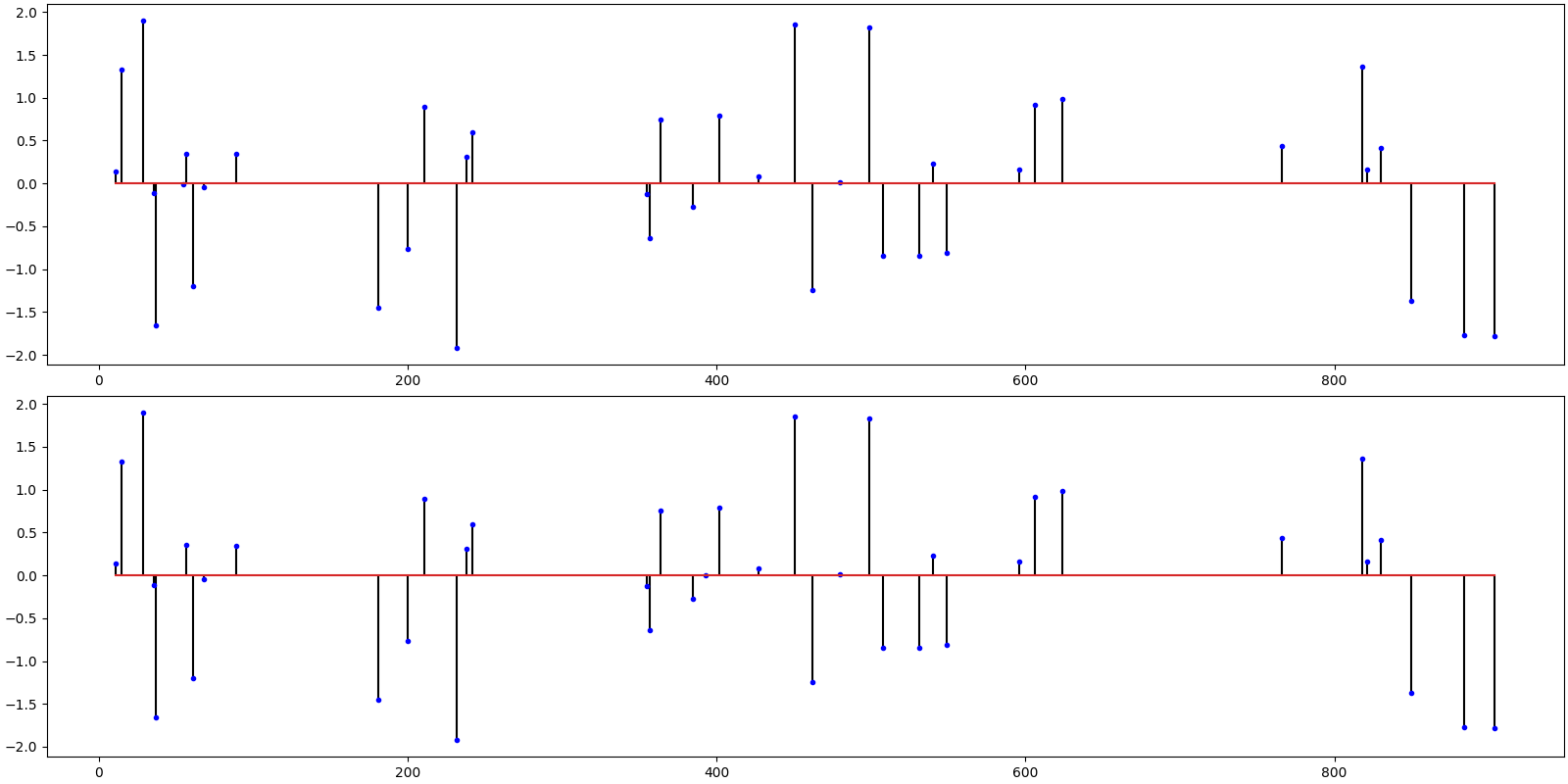
# Plot the original and the reconstructed signal
ax = crplots.h_plots(2)
crplots.plot_sparse_signals(ax, x, x_hat)

iterations 7
m=256, n=1024, k=40
r_norm 4.468207e-14
x_norm 2.590201e+01
SNR: 296.00 dB, PRD: 0 %

Subspace Pursuit ¶

Import the algorithm

from cr.sparse.pursuit import sp
# Solve the problem
sol =  sp.operator_solve_jit(T_normed, y, k)
print(sol)
# We need to scale the solution since the measurements were unscaled
x_hat = sol.x * d_scale
# Compute the SNR and PRD
print(f'SNR: {crn.signal_noise_ratio(x, x_hat):.2f} dB, PRD: {crn.percent_rms_diff(x, x_hat):.0f} %')
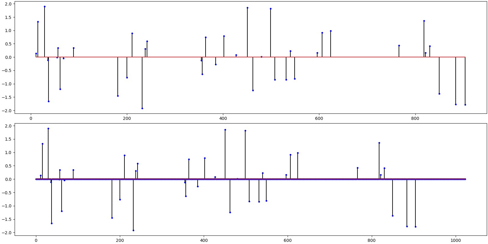
# Plot the original and the reconstructed signal
ax = crplots.h_plots(2)
crplots.plot_sparse_signals(ax, x, x_hat)

iterations 6
m=256, n=1024, k=40
r_norm 4.307734e-14
x_norm 2.590201e+01
SNR: 295.15 dB, PRD: 0 %

Hard Thresholding Pursuit ¶

Import the algorithm

from cr.sparse.pursuit import htp
# Solve the problem
sol =  htp.operator_solve_jit(T_normed, y, k)
print(sol)
# We need to scale the solution since the measurements were unscaled
x_hat = sol.x * d_scale
# Compute the SNR and PRD
print(f'SNR: {crn.signal_noise_ratio(x, x_hat):.2f} dB, PRD: {crn.percent_rms_diff(x, x_hat):.0f} %')
# Plot the original and the reconstructed signal
ax = crplots.h_plots(2)
crplots.plot_sparse_signals(ax, x, x_hat)

iterations 20
m=256, n=1024, k=40
r_norm 2.904729e-02
x_norm 2.590449e+01
SNR: 56.77 dB, PRD: 0 %

Truncated Newton Interior Points Method ¶

Import the algorithm

from cr.sparse.cvx import l1ls
# Solve the problem
# Note that this algorithm doesn't require sparsity level k as input
sol =  l1ls.solve_jit(T_normed, y, 1e-2)
print(sol)
# We need to scale the solution since the measurements were unscaled
x_hat = sol.x * d_scale
# Compute the SNR and PRD
print(f'SNR: {crn.signal_noise_ratio(x, x_hat):.2f} dB, PRD: {crn.percent_rms_diff(x, x_hat):.0f} %')
# Plot the original and the reconstructed signal
ax = crplots.h_plots(2)
crplots.plot_sparse_signals(ax, x, x_hat)

iterations 19
n_times 1121
n_trans 1121
r_norm 3.622522e-02
SNR: 51.38 dB, PRD: 0 %

Total running time of the script: (0 minutes 13.591 seconds)

Gallery generated by Sphinx-Gallery

cr-sparse

Navigation

Related Topics

Sparse Binary Sensing Matrices¶

Creating Sparse Binary Sensing Matrices ¶

Sparse Binary Sensing Linear Operators ¶

Compressive Sensing ¶

Sparse Recovery ¶

CoSaMP ¶

Subspace Pursuit ¶

Hard Thresholding Pursuit ¶

Truncated Newton Interior Points Method ¶