Random Orthogonal Measurements, Cosine Basis, ADMM

This example has following features:

• The signal being measured is not sparse by itself.

• It does have a sparse representation in discrete cosine basis.

• Measurements are taken by a partial Walsh Hadamard sensing matrix with small number of orthonormal rows

• The number of measurements is 8 times lower than the dimension of the signal space.

• ADMM based Basis pursuit denoising is being used to solve the recovery problem.

This example is adapted from YALL1 package.

Let’s import necessary libraries

import jax.numpy as jnp
from jax import random
norm = jnp.linalg.norm

import matplotlib as mpl
import matplotlib.pyplot as plt

from cr.sparse import lop
from cr.sparse.cvx.adm import yall1

Setup

# Number of measurements
m = 1024
# Ambient dimension
n = m*8

key = random.PRNGKey(0)
keys = random.split(key, 4)

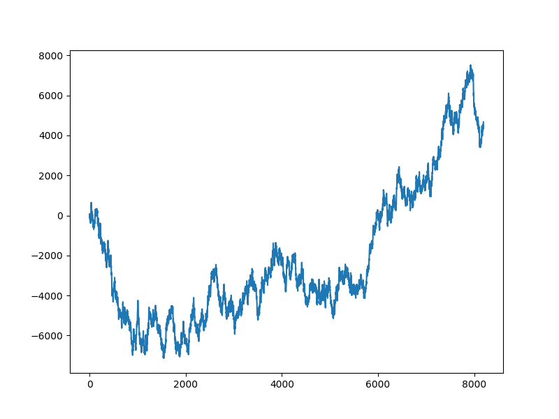
Non-sparse signal

xs = 100 * jnp.cumsum(random.normal(keys[0], (n,)))
plt.figure(figsize=(8,6), dpi= 100, facecolor='w', edgecolor='k')
plt.plot(xs)

[<matplotlib.lines.Line2D object at 0x7f27aa81c8e0>]

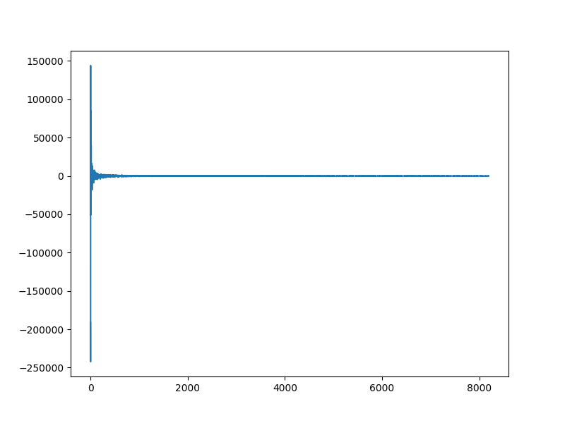
The Sparsifying Basis

Psi  = lop.jit(lop.cosine_basis(n))

alpha = Psi.trans(xs)
plt.figure(figsize=(8,6), dpi= 100, facecolor='w', edgecolor='k')
plt.plot(alpha)

[<matplotlib.lines.Line2D object at 0x7f27ab2463d0>]

Partial Walsh Hadamard Measurements Operator

# indices of the measurements to be picked
p = random.permutation(keys[1], n)
picks = jnp.sort(p[:m])
# Make sure that DC component is always picked up
picks = picks.at[0].set(0)
print(f"{picks=}")

# a random permutation of input
perm = random.permutation(keys[2], n)
print(f"{perm=}")

# Walsh Hadamard Basis operator
Twh = lop.walsh_hadamard_basis(n)

# Wrap it with picks and perm
Tpwh = lop.jit(lop.partial_op(Twh, picks, perm))

picks=Array([   0,   16,   17, ..., 8181, 8189, 8191], dtype=int64)
perm=Array([ 492, 5891, 6660, ..., 1416, 2648, 5917], dtype=int64)

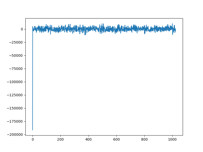
Measurement process

# Perform exact measurement
bs = Tpwh.times(xs)

# Add some noise
sigma = 0.2
noise = sigma * random.normal(keys[3], (m,))
b = bs + noise

plt.figure(figsize=(8,6), dpi= 100, facecolor='w', edgecolor='k')
plt.plot(b)

[<matplotlib.lines.Line2D object at 0x7f27ac6cf730>]

Recovery using ADMM

# tolerance for solution convergence
tol = 5e-4
# BPDN parameter
rho = 5e-4
# Run the solver
sol = yall1.solve(Tpwh, b, rho=rho, tolerance=tol, W=Psi)
iterations = int(sol.iterations)
#Number of iterations
print(f'{iterations=}')
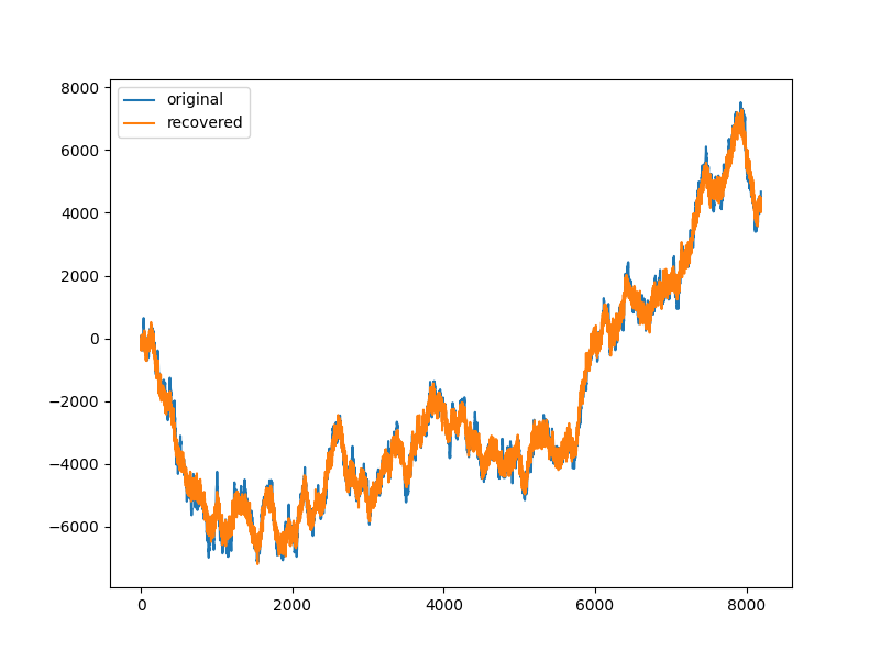
# Relative error
rel_error = norm(sol.x-xs)/norm(xs)
print(f'{rel_error=:.4e}')

iterations=192
rel_error=7.8711e-02

Solution

plt.figure(figsize=(8,6), dpi= 100, facecolor='w', edgecolor='k')
plt.plot(xs, label='original')
plt.plot(sol.x, label='recovered')
plt.legend()

<matplotlib.legend.Legend object at 0x7f27abd23760>