Recovering spikes via TNIPM

This example has following features:

• A sparse signal consists of a small number of spikes.

• The sensing matrix is a random dictionary with orthonormal rows.

• The number of measurements is one fourth of ambient dimensions.

• The measurements are corrupted by noise.

• Truncated Newton Interior Points Method (TNIPM) a.k.a. l1-ls algorithm is being used for recovery.

Let’s import necessary libraries

import jax.numpy as jnp
from jax import random
norm = jnp.linalg.norm

import matplotlib as mpl
import matplotlib.pyplot as plt

import cr.sparse as crs
import cr.sparse.data as crdata
import cr.sparse.lop as lop
import cr.sparse.cvx.l1ls as l1ls
from cr.nimble.dsp import (
  hard_threshold_by,
  support,
  largest_indices_by
)

Setup

# Number of measurements
m = 2**10
# Ambient dimension
n  = 2**12
# Number of spikes (sparsity)
k = 160
print(f'{m=}, {n=}')

key = random.PRNGKey(0)
keys = random.split(key, 4)

m=1024, n=4096

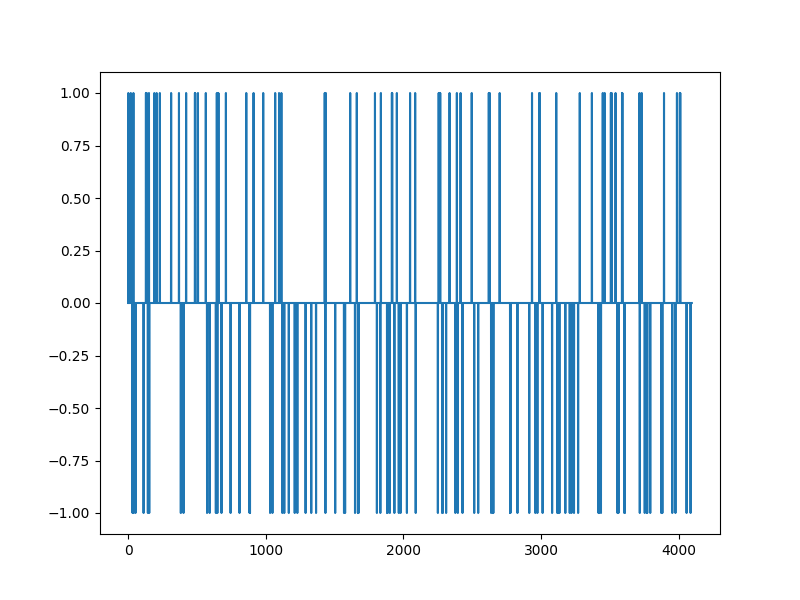
The Spikes

xs, omega = crdata.sparse_spikes(keys[0], n, k)
plt.figure(figsize=(8,6), dpi= 100, facecolor='w', edgecolor='k')
plt.plot(xs)

[<matplotlib.lines.Line2D object at 0x7f27ab240700>]

The Sparsifying Basis

A = lop.random_orthonormal_rows_dict(keys[1], m, n)

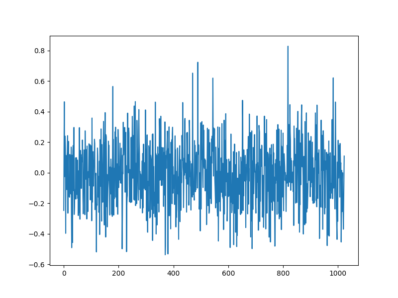
Measurement process

# Clean measurements
bs = A.times(xs)
# Noise
sigma = 0.01
noise = sigma * random.normal(keys[2], (m,))
# Noisy measurements
b = bs + noise
plt.figure(figsize=(8,6), dpi= 100, facecolor='w', edgecolor='k')
plt.plot(b)

[<matplotlib.lines.Line2D object at 0x7f27aa725f70>]

Recovery using TNIPM

# We need to estimate the regularization parameter
Atb = A.trans(b)
tau = float(0.1 * jnp.max(jnp.abs(Atb)))
print(f'{tau=}')
# Now run the solver
sol = l1ls.solve_jit(A, b, tau)

# number of L1-LS iterations
iterations = int(sol.iterations)
# number of A x operations
n_times = int(sol.n_times)
# number of A^H y operations
n_trans = int(sol.n_trans)
print(f'{iterations=} {n_times=} {n_trans=}')

# residual norm
r_norm = norm(sol.x)
print(f'{r_norm=:.3e}')

# relative error
rel_error = norm(xs - sol.x) / norm(xs)
print(f'{rel_error=:.3e}')

tau=0.05101185632358787
iterations=17 n_times=173 n_trans=174
r_norm=1.122e+01
rel_error=1.224e-01

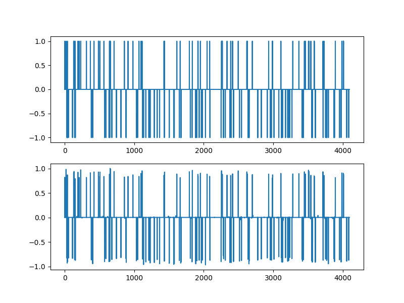
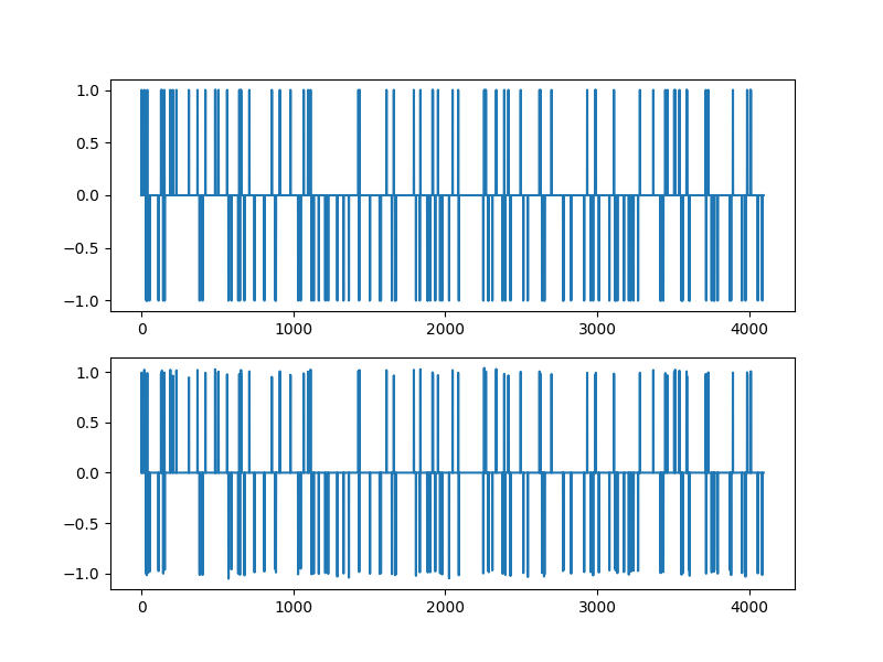
Solution

plt.figure(figsize=(8,6), dpi= 100, facecolor='w', edgecolor='k')
plt.subplot(211)
plt.plot(xs)
plt.subplot(212)
plt.plot(sol.x)

[<matplotlib.lines.Line2D object at 0x7f27aadcca00>]

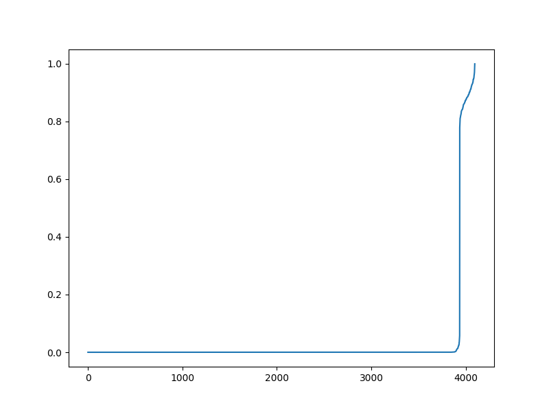
The magnitudes of non-zero values

plt.figure(figsize=(8,6), dpi= 100, facecolor='w', edgecolor='k')
plt.plot(jnp.sort(jnp.abs(sol.x)))

[<matplotlib.lines.Line2D object at 0x7f27ab063dc0>]

Thresholding for large values

x = hard_threshold_by(sol.x, 0.5)
plt.figure(figsize=(8,6), dpi= 100, facecolor='w', edgecolor='k')
plt.subplot(211)
plt.plot(xs)
plt.subplot(212)
plt.plot(x)

[<matplotlib.lines.Line2D object at 0x7f27ab22a5b0>]

Verifying the support recovery

support_xs = support(xs)
support_x = support(x)
jnp.all(jnp.equal(support_xs, support_x))

Array(True, dtype=bool)

Improvement using least squares over support

# Identify the sub-matrix of columns for the support of recovered solution's large entries
support_x = largest_indices_by(sol.x, 0.5)
AI = A.columns(support_x)
print(AI.shape)

# Solve the least squares problem over these columns
x_I, residuals, rank, s  = jnp.linalg.lstsq(AI, b)
# fill the non-zero entries into the sparse least squares solution
x_ls = jnp.zeros_like(xs)
x_ls = x_ls.at[support_x].set(x_I)

# relative error
ls_rel_error = norm(xs - x_ls) / norm(xs)
print(f'{ls_rel_error=:.3e}')

plt.figure(figsize=(8,6), dpi= 100, facecolor='w', edgecolor='k')
plt.subplot(211)
plt.plot(xs)
plt.subplot(212)
plt.plot(x_ls)

(1024, 160)
ls_rel_error=2.070e-02

[<matplotlib.lines.Line2D object at 0x7f27ab481550>]